## Diagram: Causal Graph and Jointtree Structure
### Overview
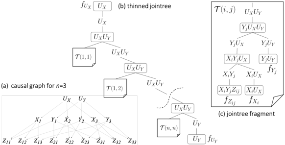
The image presents a technical diagram illustrating causal relationships and probabilistic factorization in a hierarchical model. It consists of three components:
1. **(a) Causal Graph for n=3**: A directed acyclic graph (DAG) showing variables and their dependencies.
2. **(b) Thinned Jointtree**: A factorized representation of joint probability distributions.
3. **(c) Jointtree Fragment**: A detailed subtree highlighting specific variable interactions and functions.
---
### Components/Axes
#### (a) Causal Graph for n=3
- **Nodes**:
- **X₁, X₂, X₃**: Observed variables (likely inputs or treatments).
- **Y₁, Y₂, Y₃**: Observed outcomes or responses.
- **Z₁₁, Z₁₂, Z₁₃, Z₂₁, Z₂₂, Z₂₃, Z₃₁, Z₃₂, Z₃₃**: Latent variables (confounders or mediators).
- **Edges**:
- Directed arrows from **Zᵢⱼ** to **Xᵢ** and **Yⱼ**, indicating Z variables influence both X and Y.
- No direct edges between X and Y variables, suggesting no direct causal link (Z variables mediate/confound).
#### (b) Thinned Jointtree
- **Nodes**:
- **U_X, U_Y**: Latent variables representing unobserved factors.
- **T(i,j)**: Conditional probability distributions (CPDs) parameterized by indices (i,j).
- **Structure**:
- Hierarchical factorization:
- Root nodes **U_X** and **U_Y** branch into **T(1,1)**, **T(1,2)**, ..., **T(n,n)**.
- Each **T(i,j)** node represents a conditional distribution (e.g., **P(Xᵢ, Yⱼ | U_X, U_Y)**).
#### (c) Jointtree Fragment
- **Nodes**:
- **YⱼU_XU_Y**: Composite node combining Yⱼ with latent variables.
- **XᵢYⱼZᵢⱼ**: Interaction term involving observed and latent variables.
- **XᵢU_X**: Direct dependency between Xᵢ and U_X.
- **Functions**:
- **f_UX, f_UY**: Functions mapping latent variables to distributions.
- **f_Yj, f_Zij, f_Xi**: Functions defining transformations or dependencies (e.g., **f_Zij = P(Zᵢⱼ | Xᵢ, Yⱼ)**).
---
### Detailed Analysis
#### (a) Causal Graph
- **Key Trends**:
- Z variables (**Zᵢⱼ**) act as confounders, influencing both X and Y variables.
- No direct edges between X and Y suggest no unmediated causal relationship.
#### (b) Thinned Jointtree
- **Key Trends**:
- Hierarchical decomposition of joint probability **P(X, Y, U_X, U_Y)** into conditional terms.
- **T(i,j)** nodes represent factorized components (e.g., **P(Xᵢ | U_X)**, **P(Yⱼ | U_Y)**).
#### (c) Jointtree Fragment
- **Key Trends**:
- Focus on interactions between **Xᵢ, Yⱼ, Zᵢⱼ** and latent variables.
- Functions like **f_Zij** and **f_Xi** imply conditional dependencies (e.g., **Zᵢⱼ** depends on **Xᵢ** and **Yⱼ**).
---
### Key Observations
1. **Confounder Mediation**: Z variables (**Zᵢⱼ**) mediate relationships between X and Y, consistent with causal graph assumptions.
2. **Hierarchical Factorization**: The jointtree structure decomposes the joint distribution into manageable conditional terms, enabling scalable inference.
3. **Fragment Complexity**: The jointtree fragment highlights non-trivial interactions (e.g., **XᵢYⱼZᵢⱼ**), suggesting higher-order dependencies.
---
### Interpretation
- **Causal Inference**: The diagram illustrates how latent confounders (Z) complicate causal relationships between X and Y, necessitating factorization via jointtrees.
- **Probabilistic Modeling**: The thinned jointtree and fragment demonstrate how hierarchical models (e.g., Bayesian networks) decompose complex dependencies into tractable components.
- **Uncertainty**: The absence of numerical values or error bars implies this is a conceptual diagram, not empirical data.
This structure is critical for understanding how causal graphs inform probabilistic models, particularly in scenarios with latent variables and hierarchical dependencies.