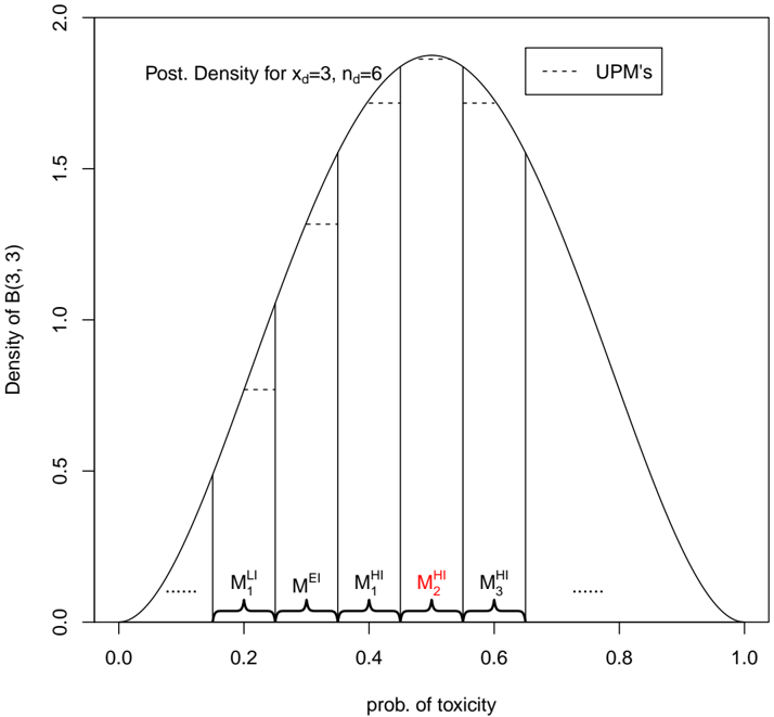
## Probability Density Chart: Posterior Density for Toxicity Probability ### Overview The image is a probability density chart showing the posterior density of a Beta distribution B(3, 3) representing the probability of toxicity. The x-axis represents the probability of toxicity, ranging from 0.0 to 1.0. The y-axis represents the density of the Beta distribution, ranging from 0.0 to 2.0. The chart also displays Uniform Prior Mass (UPM) intervals along the x-axis, marked by vertical lines and dashed horizontal lines indicating the density within each interval. ### Components/Axes * **Title:** Post. Density for x_d=3, n_d=6 * **Y-axis:** Density of B(3, 3), with scale from 0.0 to 2.0 in increments of 0.5. * **X-axis:** prob. of toxicity, with scale from 0.0 to 1.0 in increments of 0.2. * **Curve:** A bell-shaped curve representing the probability density function. * **Vertical Lines:** Represent the boundaries of the UPM intervals. * **Dashed Horizontal Lines:** Indicate the density within each UPM interval. * **UPM's Legend:** Dashed line labeled "UPM's" in a box at the top right. * **Interval Labels:** M^LI₁, M^EI, M^HI₁, M^HI₂ (red), M^HI₃ ### Detailed Analysis * **Curve Trend:** The curve is a bell-shaped curve, symmetrical around the center. It starts at approximately 0.0 at x=0.0, rises to a peak around x=0.5 with a density of approximately 1.8, and then decreases back to approximately 0.0 at x=1.0. * **UPM Intervals:** The x-axis is divided into several intervals, each representing a UPM. * M^LI₁: Located between approximately 0.1 and 0.2. * M^EI: Located between approximately 0.2 and 0.3. * M^HI₁: Located between approximately 0.3 and 0.4. * M^HI₂: Located between approximately 0.4 and 0.5. This label is in red. * M^HI₃: Located between approximately 0.5 and 0.6. * **Density within Intervals:** The dashed horizontal lines indicate the approximate density within each interval. * The density in the interval M^LI₁ is approximately 0.3. * The density in the interval M^EI is approximately 0.8. * The density in the interval M^HI₁ is approximately 1.4. * The density in the interval M^HI₂ is approximately 1.7. * The density in the interval M^HI₃ is approximately 1.7. ### Key Observations * The probability density is highest around x=0.5, indicating that the most probable value for the probability of toxicity is around 0.5. * The UPM intervals are of equal width along the x-axis. * The density within the UPM intervals increases as you move towards the center of the distribution, and then decreases as you move away from the center. * The interval M^HI₂ is highlighted in red, possibly indicating a region of interest or concern. ### Interpretation The chart visualizes the posterior probability distribution for the toxicity probability, given some observed data (x_d=3, n_d=6). The Beta distribution B(3, 3) is used as a prior, and the UPM intervals provide a way to discretize the probability space and assess the probability mass within each interval. The red highlighting of M^HI₂ suggests that this interval might be associated with a higher risk or a specific threshold of toxicity. The chart helps in understanding the uncertainty associated with the toxicity probability and in making decisions based on the available data.