## Probability Density Plot: Posterior Distribution of Toxicity Probability
### Overview
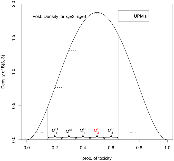
The image displays a statistical plot showing the posterior probability density function for the probability of toxicity, based on a Beta distribution with parameters (3, 3). The plot includes a main density curve, vertical reference lines marking specific points on the x-axis, and a legend. The context suggests a Bayesian analysis, likely related to dose-finding or toxicity assessment in a clinical or experimental setting.
### Components/Axes
* **Chart Type:** Probability Density Plot.
* **Main Title/Annotation:** "Post. Density for x_d=3, n_d=6" (located in the top-left quadrant of the plot area). This indicates the posterior density is calculated for a scenario with 3 observed toxicity events (`x_d=3`) out of 6 subjects or trials (`n_d=6`).
* **Y-Axis:**
* **Label:** "Density of B(3, 3)" (rotated vertically on the left side).
* **Scale:** Linear scale ranging from 0.0 to 2.0, with major tick marks at 0.0, 0.5, 1.0, 1.5, and 2.0.
* **X-Axis:**
* **Label:** "prob. of toxicity" (centered at the bottom).
* **Scale:** Linear scale ranging from 0.0 to 1.0, with major tick marks at 0.0, 0.2, 0.4, 0.6, 0.8, and 1.0.
* **Legend:**
* **Position:** Top-right corner of the plot area.
* **Content:** A dashed line symbol (`---`) followed by the text "UPM's". This likely stands for "Unbiased Probability Measures" or a similar technical term.
* **Data Series & Annotations:**
1. **Main Density Curve:** A solid, smooth, bell-shaped curve symmetric around 0.5. It represents the Beta(3,3) probability density function.
2. **Vertical Lines & Labels:** Six vertical solid lines extend from the x-axis to the density curve. Each is associated with a label below the x-axis. From left to right:
* `M₁^LI` (positioned at approximately x=0.18)
* `M^EI` (positioned at approximately x=0.28)
* `M₁^HI` (positioned at approximately x=0.38)
* `M₂^HI` (positioned at approximately x=0.48, **displayed in red font**)
* `M₃^HI` (positioned at approximately x=0.58)
* An ellipsis (`......`) is shown to the right of `M₃^HI`, near x=0.7.
3. **Dashed Horizontal Segments:** At the top of each vertical line (where it meets the density curve), there is a short, horizontal dashed line segment extending to the right. These segments are visually connected to the "UPM's" legend entry.
4. **Ellipses:** An ellipsis (`......`) is also present on the far left of the x-axis, near x=0.05, suggesting the pattern of vertical lines and labels continues beyond those explicitly shown.
### Detailed Analysis
* **Density Curve Shape:** The Beta(3,3) distribution is symmetric and unimodal, peaking at a probability of 0.5. The maximum density value at the peak is approximately 1.88 (just below the 2.0 mark on the y-axis).
* **Spatial Grounding of Labeled Points:** The labeled points (`M` values) are not evenly spaced. They are clustered more densely around the center (0.5) of the distribution. The red label `M₂^HI` is positioned very close to the distribution's mode (peak).
* **Trend Verification:** The density curve slopes upward from x=0.0 to its peak at x=0.5, then slopes downward symmetrically from x=0.5 to x=1.0. The vertical lines sample this curve at increasing x-values.
* **Approximate Data Points (Visual Estimation):**
* The density at `M₁^LI` (x≈0.18) is ~0.5.
* The density at `M^EI` (x≈0.28) is ~1.1.
* The density at `M₁^HI` (x≈0.38) is ~1.6.
* The density at `M₂^HI` (x≈0.48) is ~1.85 (near the peak).
* The density at `M₃^HI` (x≈0.58) is ~1.6.
### Key Observations
1. **Central Tendency:** The highest probability density is centered at a toxicity probability of 0.5, which is the expected value for a Beta(3,3) prior/posterior.
2. **Categorical Labels:** The subscripts (1, 2, 3) and superscripts (LI, EI, HI) on the "M" labels suggest a categorical classification system. "HI" appears most frequently. The red highlighting of `M₂^HI` indicates it is a point of particular interest or the selected value among the "HI" category.
3. **UPM Indication:** The dashed horizontal lines at the top of each vertical marker visually link these specific points on the curve to the "UPM's" concept defined in the legend.
4. **Symmetry and Spread:** The distribution is perfectly symmetric, indicating equal uncertainty about the toxicity probability being above or below 0.5. The bulk of the probability mass lies between approximately 0.2 and 0.8.
### Interpretation
This plot visualizes the updated belief (posterior distribution) about the probability of a toxic event after observing 3 events in 6 trials. The Beta(3,3) distribution suggests a prior belief that was symmetric and centered on 0.5 (a "neutral" prior), which has been updated by the data.
The labeled points (`M` values) likely represent **decision thresholds, model estimates, or recommended doses** from different methodologies or criteria (e.g., LI = Low Interest, EI = Expected Interest, HI = High Interest). The clustering of "HI" labels near the peak of the distribution suggests that methods classified as "HI" yield toxicity probability estimates that align closely with the most probable values according to the statistical model.
The red `M₂^HI` is almost certainly the **recommended or selected operating point** based on some decision rule (e.g., the median of the posterior, or a target toxicity rate). Its position near the mode reinforces that this selected value is highly consistent with the observed data.
The "UPM's" (dashed lines) likely represent a specific statistical technique (Unbiased Probability Measures) used to derive or adjust these point estimates from the continuous density curve. The plot effectively communicates both the **uncertainty** (the spread of the density curve) and the **point estimates** (the `M` values) used for decision-making in a toxicity-finding study.