## Commutative Diagram: Category Theory ### Overview The image is a commutative diagram, likely representing a relationship between objects and morphisms in category theory. It shows various objects labeled with K^T and expressions involving functions f, g, and π, connected by arrows labeled "sp", "can", and "π!". The diagram illustrates how different compositions of functions and transformations relate to each other. ### Components/Axes * **Objects:** The objects in the diagram are represented by expressions of the form K^T(…), where the content inside the parentheses varies. These include: * K^T(Z((f+g) o π)) (top-left) * K^T(Z(f o π)) (top-right) * K^T(Z(f+g)) (bottom-left) * K^T(Z(f)) (bottom-right) * K^T(Y, (f+g) o π) (middle-left, top) * K^T(Y, f o π) (middle-right, top) * K^T(X, f+g) (middle-left, bottom) * K^T(X, f) (middle-right, bottom) * **Morphisms (Arrows):** The arrows represent morphisms (transformations) between the objects. The arrows are labeled as follows: * "sp": Represents a specific transformation, appearing horizontally at the top, middle, and bottom of the diagram. * "can": Represents a canonical transformation, appearing diagonally from the top-left to middle-right, top; top-left to bottom-right; bottom-left to middle-right, bottom; and bottom-left to top-right. * "π!": Represents a transformation related to π, appearing vertically on the left and right sides of the diagram. ### Detailed Analysis * **Top Row:** The top row shows a transformation from K^T(Z((f+g) o π)) to K^T(Z(f o π)) via the morphism "sp". There is also a diagonal arrow labeled "can" from K^T(Z((f+g) o π)) to K^T(Y, f o π). * **Middle Rows:** The middle rows show transformations from K^T(Y, (f+g) o π) to K^T(Y, f o π) and from K^T(X, f+g) to K^T(X, f), both via the morphism "sp". There are also vertical arrows labeled "π!" from K^T(X, f+g) to K^T(Y, (f+g) o π) and from K^T(X, f) to K^T(Y, f o π). * **Bottom Row:** The bottom row shows a transformation from K^T(Z(f+g)) to K^T(Z(f)) via the morphism "sp". There is also a diagonal arrow labeled "can" from K^T(Z(f+g)) to K^T(X, f). * **Vertical Transformations:** The vertical transformations labeled "π!" connect K^T(Z((f+g) o π)) to K^T(Z(f+g)) on the left and K^T(Z(f o π)) to K^T(Z(f)) on the right. ### Key Observations * The diagram is structured in a rectangular grid, with transformations occurring horizontally, vertically, and diagonally. * The "sp" morphisms seem to simplify the expressions inside the K^T(…) by removing the "+g" component. * The "can" morphisms appear to be canonical mappings between different objects. * The "π!" morphisms connect objects with and without the Z prefix. ### Interpretation The diagram likely represents a commutative relationship in category theory. The commutativity implies that following different paths between two objects in the diagram results in the same transformation. The diagram seems to illustrate how the functions f, g, and π interact within the context of the K^T functor. The "sp" morphisms might represent a specialization or simplification process, while the "can" morphisms represent canonical mappings. The "π!" morphisms likely relate to a projection or pullback operation involving π. The diagram's structure suggests a careful arrangement of objects and morphisms to demonstrate a specific property or theorem within the category.

## Mathematical Commutative Diagram: Functorial Relationships ### Overview The image displays a commutative diagram from advanced mathematics, likely within category theory, homological algebra, or algebraic topology. It illustrates the relationships between several functorial constructions, denoted by `K^T`, applied to different combinations of objects (`X`, `Y`, `Z`) and morphisms or functions (`f`, `g`). The diagram is structured as a rectangular grid with six nodes connected by directed arrows, each labeled with a specific map or transformation (`sp`, `can`, `π'`). ### Components/Axes The diagram consists of six nodes arranged in two rows and three columns, with the central column containing two vertically stacked nodes. **Nodes (from top-left, moving right and down):** 1. **Top-Left:** `K^T(Z((f + g) ∘ π))` 2. **Top-Center:** `K^T(Y, (f + g) ∘ π)` 3. **Top-Right:** `K^T(Z(f ∘ π))` 4. **Bottom-Left:** `K^T(Z(f + g))` 5. **Bottom-Center:** `K^T(X, f + g)` 6. **Bottom-Right:** `K^T(Z(f))` **Arrows and Labels:** * **Horizontal Arrows (labeled `sp`):** * From `K^T(Z((f + g) ∘ π))` to `K^T(Z(f ∘ π))` (Top row, left to right). * From `K^T(Y, (f + g) ∘ π)` to `K^T(Y, f ∘ π)` (Top-center to a node not explicitly drawn but implied by the arrow's endpoint, which is `K^T(Y, f ∘ π)`). * From `K^T(X, f + g)` to `K^T(X, f)` (Bottom-center to a node not explicitly drawn but implied by the arrow's endpoint, which is `K^T(X, f)`). * From `K^T(Z(f + g))` to `K^T(Z(f))` (Bottom row, left to right). * **Diagonal Arrows (labeled `can`):** * From `K^T(Z((f + g) ∘ π))` to `K^T(Y, (f + g) ∘ π)` (Top-left to top-center). * From `K^T(Z(f ∘ π))` to `K^T(Y, f ∘ π)` (Top-right to the implied top-center-right node). * From `K^T(Z(f + g))` to `K^T(X, f + g)` (Bottom-left to bottom-center). * From `K^T(Z(f))` to `K^T(X, f)` (Bottom-right to the implied bottom-center-right node). * **Vertical Arrows (labeled `π'`):** * From `K^T(Y, (f + g) ∘ π)` to `K^T(X, f + g)` (Top-center to bottom-center). * From `K^T(Y, f ∘ π)` to `K^T(X, f)` (Implied top-center-right to implied bottom-center-right). * From `K^T(Z((f + g) ∘ π))` to `K^T(Z(f + g))` (Top-left to bottom-left). * From `K^T(Z(f ∘ π))` to `K^T(Z(f))` (Top-right to bottom-right). ### Detailed Analysis The diagram is a network of commutative squares and triangles. The primary structure is a large outer rectangle whose corners are the four `Z`-nodes. Inside this, a smaller rectangle is formed by the `Y` and `X` nodes. The arrows define specific pathways between these constructions. * **`sp` arrows:** These horizontal arrows likely represent a "specialization" or "splitting" map, transforming a construction involving a sum `(f + g)` into one involving only `f`. * **`can` arrows:** These diagonal arrows likely represent "canonical" maps, relating constructions on the object `Z` to corresponding constructions on objects `Y` or `X`. * **`π'` arrows:** These vertical arrows likely represent a map induced by a projection `π`, relating constructions involving `(f + g) ∘ π` or `f ∘ π` to those involving `f + g` or `f` directly. The diagram asserts that all paths from a given starting node to a given ending node are equivalent. For example, the path from `K^T(Z((f + g) ∘ π))` to `K^T(X, f + g)` can be taken either via `can` then `π'`, or via `π'` then `can`. The commutativity of the diagram is the key mathematical statement. ### Key Observations 1. **Symmetry:** The diagram exhibits a high degree of symmetry. The left half deals with the sum `(f + g)`, while the right half deals with the single function `f`. The top row involves composition with `π`, while the bottom row does not. 2. **Implied Nodes:** Two nodes (`K^T(Y, f ∘ π)` and `K^T(X, f)`) are not explicitly drawn as boxes but are clearly implied as the targets of multiple arrows. This is a common shorthand in such diagrams. 3. **Consistent Labeling:** The labels `sp`, `can`, and `π'` are used consistently for all arrows of the same orientation and type, indicating they represent the same kind of natural transformation or functorial map applied in different contexts. ### Interpretation This diagram is a formal, visual proof of the compatibility between several natural transformations (`sp`, `can`, `π'`) acting on a functor `K^T`. It demonstrates that the operations of "adding functions" (`f + g`), "composing with a projection" (`∘ π`), and applying the canonical and specialization maps all interact in a coherent, predictable way. The commutativity ensures that the mathematical structures are well-behaved. For instance, it shows that the process of first specializing a sum of composed functions and then projecting is the same as first projecting the sum and then specializing. Such diagrams are fundamental in areas like derived functors, spectral sequences, or the study of model categories, where tracking how different operations interact is crucial. The diagram encapsulates a complex set of relationships into a single, verifiable geometric statement.

## Diagram Type: Flowchart ### Overview The image depicts a flowchart with various nodes and arrows indicating the flow of information or processes. The chart includes mathematical expressions and symbols, suggesting it is related to a mathematical or scientific concept. ### Components/Axes - **Nodes**: Represent different stages or elements in the process. - **Arrows**: Indicate the direction of flow or relationship between nodes. - **Mathematical Expressions**: Include symbols such as \( K^T \), \( (f + g) \), \( \pi \), and \( sp \), which are likely related to transformations or operations in a mathematical context. ### Detailed Analysis or ### Content Details - The flowchart starts with \( K^T(Z(f + g)) \) and ends with \( K^T(Z(f)) \), suggesting a transformation process. - There are multiple intermediate steps involving \( K^T \) applied to different functions and variables. - The expressions \( (f + g) \) and \( \pi \) are used in the transformations, indicating possible operations like addition and a projection or mapping. ### Key Observations - The flowchart appears to be a step-by-step process for transforming a function \( Z \) using \( K^T \). - The use of \( sp \) suggests a specific type of transformation or mapping. - The presence of \( \pi \) might indicate a projection or a mapping to a lower-dimensional space. ### Interpretation The flowchart demonstrates a mathematical transformation process where a function \( Z \) is transformed using \( K^T \) and possibly a projection or mapping indicated by \( \pi \). The final result is \( K^T(Z(f)) \), which suggests that the transformation is applied to the function \( Z \) with the input \( f \). The use of \( sp \) could imply a specific type of transformation or mapping that is detailed in the context of the mathematical or scientific concept being represented.

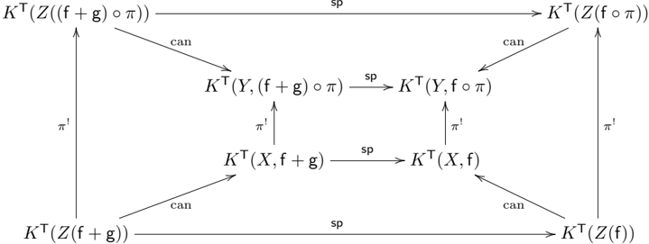
## Diagram Type: Mathematical Commutative Diagram ### Overview This image presents a complex mathematical commutative diagram, likely from the field of algebraic topology or algebraic geometry, specifically involving K-theory (`K^T`). The diagram has a three-dimensional, cube-like or prism-like structure, showing relationships between various K-theory groups. The nodes are mathematical expressions, and the directed edges (arrows) represent maps or homomorphisms between these groups. ### Components **Nodes (Vertices):** The diagram consists of eight nodes, which are K-theory groups. They are arranged in two layers, a "front" layer and a "back" layer, each forming a square. * **Back Layer (Top and Bottom):** * Top-Left: `K^T(Z((f + g) ∘ π))` * Top-Right: `K^T(Z(f ∘ π))` * Bottom-Left: `K^T(Z(f + g))` * Bottom-Right: `K^T(Z(f))` * **Front Layer (Middle):** * Upper-Left: `K^T(Y, (f + g) ∘ π)` * Upper-Right: `K^T(Y, f ∘ π)` * Lower-Left: `K^T(X, f + g)` * Lower-Right: `K^T(X, f)` **Edges (Arrows) and Labels:** The arrows represent maps between the nodes. They are labeled with specific symbols indicating the type of map. * **Horizontal Arrows (labeled 'sp'):** These arrows connect the left side of the diagram to the right side. * Top (Back): `K^T(Z((f + g) ∘ π)) —sp→ K^T(Z(f ∘ π))` * Upper (Front): `K^T(Y, (f + g) ∘ π) —sp→ K^T(Y, f ∘ π)` * Lower (Front): `K^T(X, f + g) —sp→ K^T(X, f)` * Bottom (Back): `K^T(Z(f + g)) —sp→ K^T(Z(f))` * **Vertical Arrows (labeled 'π!'):** These arrows connect the bottom nodes to the top nodes within the back layer, and the lower nodes to the upper nodes within the front layer. * Left (Back): `K^T(Z(f + g)) —π!→ K^T(Z((f + g) ∘ π))` * Right (Back): `K^T(Z(f)) —π!→ K^T(Z(f ∘ π))` * Left (Front): `K^T(X, f + g) —π!→ K^T(Y, (f + g) ∘ π)` * Right (Front): `K^T(X, f)` —π!→ `K^T(Y, f ∘ π)` * **Diagonal Arrows (labeled 'can'):** These arrows connect the back layer to the front layer. * Top-Left (Back to Front): `K^T(Z((f + g) ∘ π)) —can→ K^T(Y, (f + g) ∘ π)` * Top-Right (Back to Front): `K^T(Z(f ∘ π)) —can→ K^T(Y, f ∘ π)` * Bottom-Left (Back to Front): `K^T(Z(f + g)) —can→ K^T(X, f + g)` * Bottom-Right (Back to Front): `K^T(Z(f))` —can→ `K^T(X, f)` ### Detailed Analysis of Commutative Squares The diagram is composed of several commuting squares, which is the defining property of a commutative diagram. This means that any two paths between the same start and end nodes yield the same composition of maps. 1. **Top Face (Back and Front Upper nodes):** * Path 1: `K^T(Z((f + g) ∘ π)) —sp→ K^T(Z(f ∘ π)) —can→ K^T(Y, f ∘ π)` * Path 2: `K^T(Z((f + g) ∘ π)) —can→ K^T(Y, (f + g) ∘ π) —sp→ K^T(Y, f ∘ π)` * Commutativity: `can ∘ sp = sp ∘ can` 2. **Bottom Face (Back and Front Lower nodes):** * Path 1: `K^T(Z(f + g)) —sp→ K^T(Z(f)) —can→ K^T(X, f)` * Path 2: `K^T(Z(f + g)) —can→ K^T(X, f + g) —sp→ K^T(X, f)` * Commutativity: `can ∘ sp = sp ∘ can` 3. **Left Face (Back and Front Left nodes):** * Path 1: `K^T(Z(f + g)) —π!→ K^T(Z((f + g) ∘ π)) —can→ K^T(Y, (f + g) ∘ π)` * Path 2: `K^T(Z(f + g)) —can→ K^T(X, f + g) —π!→ K^T(Y, (f + g) ∘ π)` * Commutativity: `can ∘ π! = π! ∘ can` 4. **Right Face (Back and Front Right nodes):** * Path 1: `K^T(Z(f)) —π!→ K^T(Z(f ∘ π)) —can→ K^T(Y, f ∘ π)` * Path 2: `K^T(Z(f)) —can→ K^T(X, f) —π!→ K^T(Y, f ∘ π)` * Commutativity: `can ∘ π! = π! ∘ can` 5. **Back Face:** * Path 1: `K^T(Z(f + g)) —π!→ K^T(Z((f + g) ∘ π)) —sp→ K^T(Z(f ∘ π))` * Path 2: `K^T(Z(f + g)) —sp→ K^T(Z(f)) —π!→ K^T(Z(f ∘ π))` * Commutativity: `sp ∘ π! = π! ∘ sp` 6. **Front Face:** * Path 1: `K^T(X, f + g) —π!→ K^T(Y, (f + g) ∘ π) —sp→ K^T(Y, f ∘ π)` * Path 2: `K^T(X, f + g) —sp→ K^T(X, f) —π!→ K^T(Y, f ∘ π)` * Commutativity: `sp ∘ π! = π! ∘ sp` ### Key Observations * The diagram is highly symmetrical. * Parallel arrows always carry the same label (`sp`, `π!`, or `can`). * The structure suggests a compatibility between three types of operations: specialization (`sp`), pushforward/Gysin map (`π!`), and a canonical map (`can`). ### Interpretation This diagram illustrates the compatibility of different maps in K-theory. * `K^T(...)` likely denotes the K-theory of a space or a pair of spaces, possibly equivariant K-theory given the `T` superscript (often used for a torus action). * The arguments `X`, `Y`, `Z` are likely spaces or schemes. * `f` and `g` are likely functions or sections of bundles over these spaces. * `π` is likely a map between spaces, e.g., `π: Y → X` or `π: Z → something`. The presence of `π!` suggests it's a proper map or one for which a Gysin map is defined. * `∘` denotes the composition of functions. * `sp` likely stands for a "specialization" map, possibly related to deformation to the normal cone or a similar construction. * `π!` is a pushforward or Gysin map induced by `π`. * `can` represents a "canonical" map, which could be a restriction map, an inclusion, or another natural transformation between the K-theory groups. The overall diagram asserts that these three types of maps—specialization, pushforward, and the canonical map—commute with each other in the given context. This is a powerful statement about the naturality and consistency of these constructions in K-theory.

## Diagram: Function Composition and Transformation Flow ### Overview The diagram illustrates a structured flow of function transformations and compositions, represented by nodes labeled with mathematical expressions involving `K^T` (likely a transformation or kernel function) and arrows labeled "can" (capability) and "sp" (specialization). The structure suggests dependencies or possible paths between transformed states of functions `f`, `g`, and `π` across variables `X`, `Y`, `Z`. ### Components/Axes - **Nodes**: - `K^T(Z(f + g)∘π)` (top-left) - `K^T(Y, f∘π)` (top-right) - `K^T(X, f + g)` (middle-left) - `K^T(X, f)` (middle-right) - `K^T(Z(f + g))` (bottom-left) - `K^T(Z(f))` (bottom-right) - **Arrows**: - Vertical arrows labeled `π'` (prime symbol) connect nodes across rows. - Horizontal arrows labeled "sp" or "can" connect nodes within rows. - **Labels**: - `π'` appears on vertical arrows, suggesting a derivative or transformed version of `π`. - `sp` and "can" likely denote operational relationships (e.g., specialization, capability). ### Detailed Analysis 1. **Top Row**: - `K^T(Z(f + g)∘π)` → `K^T(Y, f∘π)` via "sp" (specialization). - `K^T(Z(f + g)∘π)` → `K^T(Z(f∘π))` via "can" (capability). 2. **Middle Row**: - `K^T(X, f + g)` → `K^T(X, f)` via "sp". - `K^T(Y, f∘π)` → `K^T(Z(f∘π))` via "can". 3. **Bottom Row**: - `K^T(Z(f + g))` → `K^T(Z(f))` via "sp". 4. **Vertical Connections**: - All nodes in a column are connected by `π'` arrows, implying a shared transformation axis. ### Key Observations - **Specialization ("sp")**: Used for horizontal transitions, possibly indicating refinement or narrowing of function scope (e.g., `f + g` → `f`). - **Capability ("can")**: Used for vertical transitions, suggesting broader applicability or existence of paths (e.g., `Z(f + g)∘π` → `Z(f∘π)`). - **Prime Symbol (`π'`)**: Indicates a transformed or derived version of `π`, possibly a derivative or adjusted parameter. - **Function Composition**: The `∘` operator denotes function composition (e.g., `f∘π` means `f` applied after `π`). ### Interpretation The diagram likely models a system where functions `f`, `g`, and `π` undergo transformations across variables `X`, `Y`, `Z`. The "sp" and "can" labels suggest a framework for reasoning about possible transformations (e.g., in category theory, functional programming, or optimization). For example: - **Specialization** (`sp`) may represent deterministic or constrained transformations (e.g., simplifying `f + g` to `f`). - **Capability** (`can`) may indicate non-deterministic or optional paths (e.g., adapting `Z(f + g)∘π` to `Z(f∘π)`). - The vertical `π'` connections imply a shared transformation layer across all nodes, possibly a global parameter or constraint. This structure could represent a proof system, computational graph, or theoretical model for function behavior under composition and transformation.