## Diagram: State Transition Diagrams with Annotations
### Overview
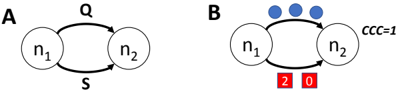
The image displays two side-by-side diagrams, labeled **A** and **B**, illustrating relationships between two nodes, `n1` and `n2`. Diagram A shows a basic bidirectional connection, while Diagram B adds quantitative and categorical annotations to a similar structure.
### Components/Axes
* **Diagram A (Left):**
* **Nodes:** Two circles labeled `n1` (left) and `n2` (right).
* **Edges:** Two directed, curved arrows connecting the nodes.
* Top arrow: Labeled `Q`, points from `n1` to `n2`.
* Bottom arrow: Labeled `S`, points from `n2` to `n1`.
* **Diagram B (Right):**
* **Nodes:** Two circles labeled `n1` (left) and `n2` (right).
* **Edges:** Two directed, curved arrows connecting the nodes.
* **Annotations:**
* **Above the top edge:** Three solid blue circles arranged horizontally.
* **Below the bottom edge:** Two solid red squares arranged horizontally. The left square contains the white numeral `2`. The right square contains the white numeral `0`.
* **Text Label:** The text `ccc=1` is positioned to the upper-right of node `n2`.
### Detailed Analysis
* **Diagram A Structure:** Represents a simple, symmetric, two-state system with two possible transitions: `Q` (from state `n1` to `n2`) and `S` (from state `n2` to `n1`).
* **Diagram B Structure:** Maintains the same core node-and-edge topology as Diagram A but introduces additional data layers:
1. **Blue Circles (Top Edge):** Three identical blue circles are associated with the transition from `n1` to `n2`. Their meaning is not explicitly labeled but could represent a count, weight, or categorical attribute.
2. **Red Squares with Numbers (Bottom Edge):** Two red squares are associated with the transition from `n2` to `n1`. They contain explicit numerical values: `2` and `0`. This suggests a quantitative measure, possibly a cost, capacity, or score split into two components.
3. **`ccc=1` Label:** This is a discrete parameter or variable assignment associated with node `n2` or the system state represented by Diagram B.
### Key Observations
1. **Structural Consistency:** Both diagrams share an identical core layout of nodes and directional edges, establishing a clear visual comparison.
2. **Information Density:** Diagram B is significantly more information-dense than Diagram A, adding three visual elements (blue circles, red squares) and one textual parameter (`ccc=1`).
3. **Color Coding:** A clear color distinction is used: blue for the top-edge annotations and red for the bottom-edge annotations. The numbers within the red squares are white for contrast.
4. **Spatial Grounding:** All annotations are placed in close proximity to their associated edges, creating a clear visual link. The `ccc=1` label is spatially associated with the right side of the diagram, near `n2`.
### Interpretation
These diagrams likely model a **state machine, Markov chain, or a simple network flow**. Diagram A defines the basic possible transitions between two states (`n1` and `n2`). Diagram B enriches this model with specific parameters:
* The **three blue circles** could indicate that the transition `n1 -> n2` has a multiplicity of 3, a weight of 3, or is associated with three discrete units of a resource.
* The **red squares with `2` and `0`** suggest the transition `n2 -> n1` has a composite cost or value. For example, it might incur a cost of 2 in one dimension and 0 in another, or have a capacity of 2 with 0 currently used.
* The parameter **`ccc=1`** sets a global condition or a property of state `n2` for the scenario depicted in B.
The progression from A to B demonstrates how a simple relational model is augmented with quantitative and categorical data for analysis, simulation, or optimization purposes. The diagrams serve as a visual schema for a system where the movement between two states is governed by labeled rules (`Q`, `S`) and measured by specific metrics.