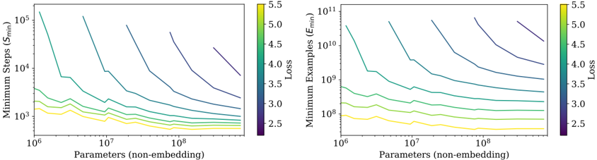
## Dual Line Charts: Scaling Laws for Minimum Training Steps and Examples vs. Model Size ### Overview The image displays two side-by-side line charts on a white background. Both charts plot a metric related to training efficiency (y-axis) against model size (x-axis) on logarithmic scales. Each chart contains multiple colored lines, with the color corresponding to a specific "Loss" value as indicated by a shared color bar legend. The charts illustrate scaling laws, showing how the minimum resources required for training change as model parameters increase. ### Components/Axes **Shared Elements:** * **X-Axis (Both Charts):** Label: `Parameters (non-embedding)`. Scale: Logarithmic, ranging from `10^6` to `10^8`. Major tick marks are at `10^6`, `10^7`, and `10^8`. * **Color Bar Legend (Right of each chart):** A vertical bar labeled `Loss` at the top. The scale runs from `2.5` (bottom, dark purple) to `5.5` (top, bright yellow). The gradient transitions through blue, teal, and green. This legend maps line color to a specific loss value. **Left Chart:** * **Title/Y-Axis Label:** `Minimum Steps (S_min)`. * **Y-Axis Scale:** Logarithmic, ranging from `10^3` to `10^5`. Major tick marks are at `10^3`, `10^4`, and `10^5`. **Right Chart:** * **Title/Y-Axis Label:** `Minimum Examples (E_min)`. * **Y-Axis Scale:** Logarithmic, ranging from `10^8` to `10^11`. Major tick marks are at `10^8`, `10^9`, `10^10`, and `10^11`. ### Detailed Analysis **Left Chart (Minimum Steps vs. Parameters):** * **Trend Verification:** All lines slope downward from left to right, indicating that as the number of parameters increases, the minimum number of training steps required to achieve a given loss decreases. * **Data Series (from top to bottom, corresponding to increasing Loss):** * **Dark Purple Line (Loss ≈ 2.5):** Starts highest on the y-axis (near `10^5` steps at `10^6` parameters) and shows the steepest decline. * **Blue/Teal Lines (Loss ≈ 3.0 - 4.0):** Occupy the middle region. Their slopes are less steep than the dark purple line. * **Green/Yellow Lines (Loss ≈ 4.5 - 5.5):** Start lowest on the y-axis (near `10^3` steps at `10^6` parameters) and have the shallowest slopes. The yellow line (Loss ≈ 5.5) is nearly flat. * **Key Data Points (Approximate):** * For a target Loss of ~2.5 (dark purple), training steps drop from ~100,000 (`10^5`) for a 1M parameter model to ~10,000 (`10^4`) for a 100M parameter model. * For a target Loss of ~5.5 (yellow), training steps remain consistently low, around 1,000-2,000 (`10^3`), across the entire parameter range. **Right Chart (Minimum Examples vs. Parameters):** * **Trend Verification:** All lines also slope downward from left to right, showing that larger models require fewer training examples to reach a target loss. * **Data Series (from top to bottom, corresponding to increasing Loss):** * **Dark Purple Line (Loss ≈ 2.5):** Starts extremely high (near `10^11` examples at `10^6` parameters) and declines steeply. * **Blue/Teal Lines (Loss ≈ 3.0 - 4.0):** Show a clear, consistent downward slope. * **Green/Yellow Lines (Loss ≈ 4.5 - 5.5):** Start much lower (near `10^8` examples) and have very shallow slopes, with the yellow line (Loss ≈ 5.5) being almost horizontal. * **Key Data Points (Approximate):** * For a target Loss of ~2.5 (dark purple), the required examples drop from ~100 billion (`10^11`) for a 1M parameter model to ~10 billion (`10^10`) for a 100M parameter model. * For a target Loss of ~5.5 (yellow), the required examples stay relatively constant at around 100 million (`10^8`). ### Key Observations 1. **Inverse Power-Law Relationship:** Both charts demonstrate a clear inverse power-law relationship between model size and the minimum training resources (steps or examples) needed to achieve a fixed loss. The lines are roughly straight on log-log plots. 2. **Loss as a Vertical Shift:** The "Loss" value primarily acts as a vertical shift on the log-log plot. Higher loss targets (yellow lines) require exponentially fewer steps and examples than lower loss targets (purple lines) for the same model size. 3. **Convergence of Slopes:** The slopes of the lines for different loss values are not parallel. The lines for lower loss (purple) are steeper, meaning the benefit of scaling up model size (in terms of reducing required steps/examples) is more pronounced when aiming for very high performance (low loss). 4. **Plateauing for High Loss:** For very high loss targets (e.g., 5.5), the curves flatten significantly, especially in the "Minimum Steps" chart. This suggests that beyond a certain model size (~10^7 parameters), further scaling provides negligible reduction in the already minimal steps needed to achieve poor performance. ### Interpretation These charts visualize fundamental **scaling laws** in machine learning, specifically relating model size, training data, and compute (steps) to final performance (loss). * **The Efficiency-Performance Trade-off:** The data quantifies a core trade-off: achieving lower loss (better performance) is exponentially more expensive in terms of both training steps and data examples. A model targeting Loss=2.5 requires orders of magnitude more resources than one targeting Loss=4.5. * **The Value of Scale for High Performance:** The steeper slopes for low-loss lines indicate that **scaling model parameters is most beneficial when you are pushing for state-of-the-art performance**. For a fixed compute budget (steps), increasing model size allows you to achieve a lower loss. Conversely, for a fixed low loss target, scaling the model reduces the required compute. * **Implications for Training Strategy:** The charts suggest different optimal strategies. If the goal is a quick, rough model (high loss), a small model with a modest dataset suffices. If the goal is a high-performance model (low loss), investing in a very large model and a massive dataset is not just beneficial but necessary, as the resource requirements scale down favorably with model size in that regime. * **Peircean Insight:** The charts are an **abductive** reasoning tool. They don't just show data; they suggest an underlying principle: the process of neural network learning follows predictable, quantifiable laws where data, compute, and model capacity are interchangeable currencies to a degree, governed by power laws. This allows for extrapolation and planning of large-scale training runs.