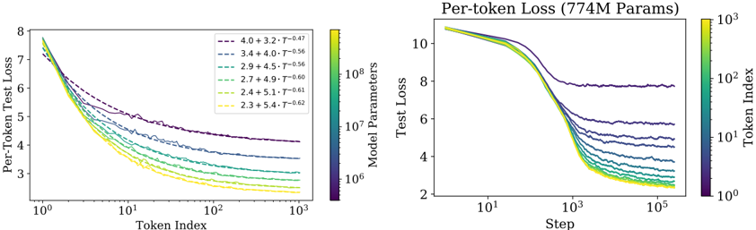
## Line Graphs: Per-Token Test Loss vs. Token Index and Step
### Overview
The image contains two side-by-side line graphs comparing per-token test loss across different model configurations. The left graph plots loss against token index (log scale), while the right graph plots loss against training steps (log scale). Both graphs use color-coded lines to represent model parameters and training-related variables.
### Components/Axes
**Left Graph (Per-Token Test Loss):**
- **X-axis**: Token Index (log scale, 10⁰ to 10³)
- **Y-axis**: Per-Token Test Loss (2 to 8)
- **Legend**:
- Line styles/colors represent combinations of model parameters (4.0, 3.4, 2.9, 2.7, 2.4, 2.3) and T values (3.2, 4.0, 4.5, 4.9, 5.1, 5.4)
- Example: "4.0 + 3.2 - T^0.47" (dashed purple line)
- **Color Bar**: Not present (legend uses discrete colors)
**Right Graph (Per-token Loss, 774M Params):**
- **X-axis**: Step (log scale, 10¹ to 10⁵)
- **Y-axis**: Test Loss (2 to 10)
- **Legend**:
- Color gradient from yellow (10³) to purple (10⁸) representing model parameters
- No explicit labels for individual lines
### Detailed Analysis
**Left Graph Trends:**
1. All lines show decreasing loss as token index increases, with steeper declines at lower token indices.
2. Lines with higher T values (e.g., 5.4) have shallower slopes compared to lower T values (e.g., 3.2).
3. Model parameter values (4.0 vs. 2.3) correlate with initial loss magnitude: higher parameters start with lower loss.
4. Example data points:
- "4.0 + 3.2 - T^0.47": Starts at ~7.5 loss at token index 10⁰, ends at ~4.2 at 10³
- "2.3 + 5.4 - T^0.62": Starts at ~7.8 loss, ends at ~3.0 at 10³
**Right Graph Trends:**
1. All lines show rapid initial loss reduction (steps 10¹–10³), then plateau.
2. Higher parameter models (yellow) maintain lower loss than lower parameter models (purple).
3. Example data points:
- 10³ parameters: Loss drops from ~10 to ~4 by step 10³
- 10⁸ parameters: Loss drops from ~10 to ~2.5 by step 10⁵
### Key Observations
1. **Log Scale Impact**: Both axes use logarithmic scales, emphasizing performance at extreme values (early tokens/steps and large parameter counts).
2. **Parameter Efficiency**: Higher parameter models (left graph's 4.0 vs. right graph's 10⁸) achieve better loss reduction.
3. **Training Dynamics**: The right graph suggests diminishing returns in loss reduction after ~10³ steps for all models.
4. **T Value Influence**: In the left graph, higher T values correlate with slower loss reduction, suggesting a trade-off between T and parameter efficiency.
### Interpretation
The data demonstrates that:
1. **Model Capacity Matters**: Larger models (higher parameters) consistently outperform smaller ones in both token index and step-based loss reduction.
2. **Training Efficiency**: Loss reduction follows a power-law decay, with most significant improvements occurring in the initial training phases (first 10³ steps/tokens).
3. **Hyperparameter Trade-offs**: The T values in the left graph appear to modulate the learning curve's steepness, potentially representing regularization or optimization parameters.
4. **Scalability Limits**: The plateauing loss in the right graph suggests diminishing returns for further training beyond ~10³ steps, regardless of model size.
The graphs collectively illustrate the relationship between model architecture (parameters), training dynamics (steps/tokens), and optimization hyperparameters (T) in determining per-token loss reduction. The color-coded legends provide critical context for comparing these multidimensional relationships.