\n
## [Chart Type]: Dual Cross-Section Line Plots
### Overview
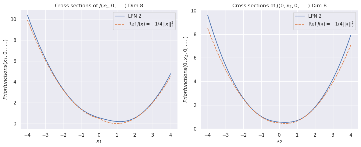
The image displays two side-by-side line charts, each showing a cross-sectional view of a function `J` in an 8-dimensional space. The left chart plots the function against the first dimension (`x₁`), while the right chart plots it against the second dimension (`x₂`). Both charts compare a learned function ("LPN 2") against a theoretical reference function.
### Components/Axes
**Titles:**
* Left Chart: `Cross sections of J(x₁, 0, ...) Dim 8`
* Right Chart: `Cross sections of J(0, x₂, 0, ...) Dim 8`
**Axes:**
* **X-Axis (Left Chart):** Label is `x₁`. Scale ranges from -4 to 4 with major tick marks at every integer (-4, -3, -2, -1, 0, 1, 2, 3, 4).
* **X-Axis (Right Chart):** Label is `x₂`. Scale ranges from -4 to 4 with major tick marks at every integer (-4, -3, -2, -1, 0, 1, 2, 3, 4).
* **Y-Axis (Both Charts):** Label is `Priorfunctions(x₁, 0, ...)` for the left chart and `Priorfunctions(0, x₂, 0, ...)` for the right chart. The scale ranges from 0 to 10 with major tick marks at 0, 2, 4, 6, 8, 10.
**Legend (Both Charts, positioned in the top-right corner):**
* **Solid Blue Line:** Label is `LPN 2`.
* **Dashed Orange Line:** Label is `Ref J(x) = -1/4||x||₂²`. This denotes a reference function defined as negative one-quarter of the squared L2 norm of the input vector `x`.
### Detailed Analysis
**Left Chart (Cross-section along x₁):**
* **Trend Verification:** Both curves form a symmetric, upward-opening parabola with a minimum near `x₁ = 1`.
* **Data Series - LPN 2 (Blue):**
* At `x₁ = -4`, the value is approximately 10.2.
* The curve descends to a minimum value of approximately 0.2 at `x₁ ≈ 1`.
* It then ascends, reaching approximately 4.8 at `x₁ = 4`.
* **Data Series - Reference (Orange Dashed):**
* At `x₁ = -4`, the value is approximately 9.8.
* The curve descends to a minimum value of approximately 0.0 at `x₁ = 1`.
* It then ascends, reaching approximately 4.5 at `x₁ = 4`.
* **Comparison:** The "LPN 2" curve closely follows the reference parabola but is consistently shifted slightly upward. The minimum of "LPN 2" is slightly above zero, while the reference function's minimum is exactly zero at `x₁=1`.
**Right Chart (Cross-section along x₂):**
* **Trend Verification:** Both curves form a symmetric, upward-opening parabola with a minimum near `x₂ = 1`.
* **Data Series - LPN 2 (Blue):**
* At `x₂ = -4`, the value is approximately 9.5.
* The curve descends to a minimum value of approximately 0.5 at `x₂ ≈ 1`.
* It then ascends, reaching approximately 8.0 at `x₂ = 4`.
* **Data Series - Reference (Orange Dashed):**
* At `x₂ = -4`, the value is approximately 8.5.
* The curve descends to a minimum value of approximately 0.4 at `x₂ ≈ 1`.
* It then ascends, reaching approximately 7.2 at `x₂ = 4`.
* **Comparison:** Similar to the left chart, "LPN 2" tracks the reference function but sits slightly above it. The vertical offset appears more pronounced at the extremes (`x₂ = ±4`) compared to the left chart.
### Key Observations
1. **Parabolic Shape:** Both cross-sections reveal that the function `J` is quadratic (parabolic) along the `x₁` and `x₂` dimensions when other dimensions are held at zero.
2. **Minimum Location:** The minimum of the function occurs at `x₁ = 1` and `x₂ = 1` for both the learned and reference functions.
3. **Model Fidelity:** The "LPN 2" model successfully captures the overall parabolic shape and location of the minimum of the reference function `J(x) = -1/4||x||₂²`.
4. **Systematic Offset:** There is a consistent, small positive offset between the "LPN 2" curve and the reference curve across both plots. This offset is not uniform; it appears slightly larger at the boundaries of the plotted range (`x = ±4`) than near the minimum.
5. **Scale Difference:** The function values at the boundaries differ between the two plots. For example, at `x = -4`, the value is ~10.2 for `x₁` but ~9.5 for `x₂`. This indicates the function's behavior is not perfectly symmetric across all dimensions, despite the reference function being rotationally symmetric (depending only on the norm).
### Interpretation
The charts demonstrate a validation or analysis of a learned model ("LPN 2") against a known theoretical prior distribution. The reference function `J(x) = -1/4||x||₂²` represents a simple, isotropic Gaussian-like prior (its negative log would be proportional to the squared norm). The fact that the cross-sections are parabolas confirms this.
The "LPN 2" model appears to be a neural network or similar function approximator trained to represent this prior. The close match indicates successful learning of the core quadratic structure. The persistent positive offset suggests the model has learned a function that is everywhere slightly higher than the target. This could be due to:
* A regularization effect during training.
* An inherent bias in the model architecture.
* The model approximating a slightly different function that includes a small constant term.
The slight asymmetry between the `x₁` and `x₂` cross-sections (different values at `x=±4`) is notable. Since the reference function is perfectly symmetric, this asymmetry must originate from the "LPN 2" model itself, indicating its learned representation is not perfectly isotropic. This could be a result of the training data, optimization path, or model capacity. Overall, the visualization confirms the model has learned the essential geometric properties of the target prior, with minor, systematic deviations.