## ReRAM Device Characteristics and Array Metrics ### Overview The image presents data on the analog switching characteristics of a ReRAM (Resistive Random-Access Memory) device in an open-loop configuration. It includes plots showing conductance changes over pulse number, statistical response of an array, and experimental array metrics related to Tiki-Taka training. ### Components/Axes **Panel a: Analog Switching Characteristics** * **Title:** Analog switching characteristics of a ReRAM device (open-loop) * **Y-axis:** Conductance [µS], with a logarithmic scale from 10 to 100. * **X-axis:** Pulse Number, ranging from 0 to 2100. * **Voltage Pulses:** A schematic at the top shows alternating positive (Vset) and negative (Vreset) voltage pulses. Vset pulses are shown in red, and Vreset pulses are shown in blue. The pulse width is 2.5µs. * **Annotations:** * "x400", "x500" indicate the number of pulses in each block. * "Sample Device: Potentiation: 1.35V, 2.5µs; Depression: 1.3V, 2.5µs" describes the pulse parameters. * **Data Series:** * A red-to-blue gradient line shows the conductance of a sample device over time. The red portion represents potentiation, and the blue portion represents depression. * **Horizontal Lines:** * A red dashed line labeled "Gmax" is at approximately 90 µS. * A blue dashed line labeled "Gmin" is at approximately 15 µS. * A yellow line labeled "Gsp" is at approximately 40 µS. * A yellow line labeled "2ΔGsp" is at approximately 40 µS. **Panel b: Array-Level Open-Loop Statistical Response** * **Title:** Array-level open-loop statistical response * **Y-axis:** Conductance [µS], with a logarithmic scale from 10 to 100. * **X-axis:** Pulse Number, ranging from 0 to 2100. * **Data Series:** * A gray shaded region represents the array experimental data. * **Vertical Line:** * A yellow dashed line is present at x = 1200. * **Annotation:** * "±σ" indicates the standard deviation around the conductance value at the yellow line. * **Inset Plot:** * **Title:** G after 1200 pulses [µS] * **Y-axis:** Probability Density, ranging from 0.0 to 1.0. * **X-axis:** G after 1200 pulses [µS], ranging from 60 to 120. * A black curve represents the probability density of the conductance after 1200 pulses. * A black dot labeled "G#1200" is at approximately 90 µS. * "±σ" indicates the standard deviation around the mean conductance value. **Panel c: Experimental Array Metrics for Tiki-Taka Training** * **Title:** Experimental array metrics for Tiki-Taka training * **Subplots (from left to right):** * **Number of States:** * **Y-axis:** Normalized Probability Density, ranging from 0.0 to 1.0. * **X-axis:** Number of States, ranging from 10 to 40. * A purple curve represents the probability density. * A black dashed line indicates the mean at 22. * "Nstates = (Gmax - Gmin) / ΔGsp" is the formula for the number of states. * Black dots represent experimental data points. * "Mean = 22" * "Exp." * **Symmetry Point Skew:** * **Y-axis:** Normalized Probability Density, ranging from 0.0 to 1.0. * **X-axis:** Symmetry Point Skew (%), ranging from 20 to 100. * A green curve represents the probability density. * A black dashed line indicates the mean at 61%. * "SPskew = (Gmax - Gsp) / (Gmax - Gmin)" is the formula for the symmetry point skew. * Green dots represent experimental data points. * "Mean = 61%" * "Exp." * **Noise to Signal Ratio:** * **Y-axis:** Normalized Probability Density, ranging from 0.0 to 1.0. * **X-axis:** Noise to Signal Ratio (%), ranging from 70 to 110. * A blue curve represents the probability density. * A black dashed line indicates the mean at 90%. * "NSR = σΔGsp / ΔGsp" is the formula for the noise-to-signal ratio. * Blue dots represent experimental data points. * "Mean = 90%" * "Exp." **8x4 ReRAM Array Diagram** * A schematic of an 8x4 ReRAM array is shown on the left side of the image. * Each cell is labeled as W(row, column), where row ranges from 1 to 8 and column ranges from 1 to 4. * The cells are colored in shades of green and purple. * The cell W(7,4) is highlighted with a yellow border. ### Detailed Analysis **Panel a:** * The conductance initially increases rapidly with the application of positive voltage pulses (potentiation), reaching a maximum value (Gmax) of approximately 90 µS. * After approximately 400 pulses, the polarity is switched to negative voltage pulses (depression), and the conductance decreases rapidly, reaching a minimum value (Gmin) of approximately 15 µS. * The conductance then fluctuates around an intermediate value (Gsp) of approximately 40 µS. **Panel b:** * The array-level data shows a similar trend to the single-device data, but with more variability, represented by the gray shaded region. * The inset plot shows the distribution of conductance values after 1200 pulses, with a mean value around 90 µS and a standard deviation of ±σ. **Panel c:** * The number of states (Nstates) has a mean value of 22. * The symmetry point skew (SPskew) has a mean value of 61%. * The noise-to-signal ratio (NSR) has a mean value of 90%. ### Key Observations * The ReRAM device exhibits analog switching behavior, with conductance values that can be continuously adjusted by applying voltage pulses. * The array-level data shows more variability than the single-device data, indicating device-to-device variations. * The experimental array metrics provide insights into the performance of the ReRAM array for Tiki-Taka training. ### Interpretation The data suggests that the ReRAM device is capable of analog switching, which is essential for implementing neuromorphic computing architectures. The array-level data highlights the importance of considering device-to-device variations when designing ReRAM-based systems. The experimental array metrics provide a quantitative assessment of the ReRAM array's performance for Tiki-Taka training, which is a specific type of machine learning algorithm. The high noise-to-signal ratio (NSR) could be a limiting factor for the performance of the ReRAM array in certain applications.

\n ## Chart: Analog Switching Characteristics of a ReRAM Device & Experimental Array Metrics ### Overview The image presents a series of charts illustrating the analog switching characteristics of a Resistive Random Access Memory (ReRAM) device, along with experimental array metrics for a "Tiki-Taka" training process. The charts explore conductance changes with pulse number, statistical response, and distributions of key parameters. The image is divided into three main sections: (a) a conductance vs. pulse number plot with inset voltage waveform, (b) an array-level open-loop statistical response plot with a probability distribution inset, and (c) three histograms showing distributions of number of states, symmetry, and noise. ### Components/Axes **Section (a):** * **Title:** Analog switching characteristics of a ReRAM device (open-loop) * **X-axis:** Pulse Number (0 to 2100) * **Y-axis:** Conductance (logarithmic scale, approximately 1 to 100 [µS]) * **Voltage Waveform (top):** Shows a series of pulses labeled 2.5µs, x400, x400, x500. The voltage is indicated as V_set. * **Annotations:** G_max, G_min, ΔG_sp. * **Sample Device:** Potentiation: 1.35V, 3.5µs; Depression: 1.3V, 2.5µs **Section (b):** * **Title:** Array-level open-loop statistical response * **X-axis:** Pulse Number (0 to 2100) * **Y-axis:** Conductance (logarithmic scale, approximately 1 to 100 [µS]) * **Inset:** Probability distribution of conductance after 1200 pulses (µS). Labeled with ±σ. * **Annotation:** Array exp. data **Section (c):** * **Title:** Experimental array metrics for Tiki-Taka training * **Histogram 1:** * **X-axis:** Number of States (0 to 31) * **Y-axis:** Normalized Probability Density (0 to 1.0) * **Annotations:** Mean = 22, n_states, Exp. * **Histogram 2:** * **X-axis:** Symmetry (0 to 1.0) * **Y-axis:** Normalized Probability Density (0 to 1.0) * **Annotations:** Mean = 61%, SP_skew = σ_max/ΔG₀, Exp. * **Histogram 3:** * **X-axis:** Noise (0 to 1.0) * **Y-axis:** Normalized Probability Density (0 to 1.0) * **Annotations:** Mean = 90%, NSR = σ_noise/ΔG₀, Exp. **Additional Element:** * **8x4 ReRAM array:** A grid labeled W_(i,j) where i ranges from 1 to 8 and j ranges from 1 to 4. ### Detailed Analysis or Content Details **Section (a):** The conductance vs. pulse number plot shows a fluctuating conductance value. The line starts at approximately 20 µS and fluctuates between approximately 20 µS and 80 µS for the first 800 pulses. After 800 pulses, the conductance generally decreases, reaching a minimum of approximately 10 µS around pulse number 1600. The conductance then increases again, reaching approximately 40 µS at pulse number 2100. G_max is approximately 80 µS and G_min is approximately 10 µS. ΔG_sp is approximately 60 µS. **Section (b):** The array-level response shows a similar trend to (a), but with a wider spread of data points. The data points are clustered around a central line that decreases from approximately 60 µS to 20 µS between pulse numbers 0 and 1600, then increases slightly to approximately 30 µS at pulse number 2100. The inset shows a probability distribution centered around approximately 70 µS with a standard deviation of approximately 10 µS. **Section (c):** * **Histogram 1 (Number of States):** The distribution is centered around 22 states, with a peak probability density of approximately 0.25. * **Histogram 2 (Symmetry):** The distribution is centered around 61% symmetry, with a peak probability density of approximately 0.3. * **Histogram 3 (Noise):** The distribution is centered around 90% noise, with a peak probability density of approximately 0.4. ### Key Observations * The conductance of the ReRAM device exhibits significant fluctuations with each pulse. * The array-level response shows a wider distribution of conductance values compared to the single device response. * The Tiki-Taka training process results in an average of 22 states, 61% symmetry, and 90% noise. * The inset in (b) shows a relatively narrow distribution of conductance values after 1200 pulses, indicating some degree of convergence. ### Interpretation The data suggests that the ReRAM device exhibits analog switching behavior, with conductance values that can be modulated by applying a series of pulses. The fluctuations in conductance may be due to stochastic effects or variations in the device characteristics. The array-level response shows that these fluctuations are amplified when multiple devices are connected in an array. The Tiki-Taka training process appears to be effective in achieving a reasonable number of states, but it also introduces a significant amount of noise. The symmetry metric indicates the balance between potentiation and depression during the training process. The high noise level may limit the precision of the analog storage. The inset in (b) suggests that the conductance distribution converges after a certain number of pulses, indicating that the device is approaching a stable state. The ReRAM array is labeled with W_(i,j), indicating a matrix of resistive elements, likely used for parallel processing or memory storage. The "Tiki-Taka" training likely refers to a specific algorithm or method used to tune the conductance levels of the ReRAM array for a particular application, potentially related to neural network training.

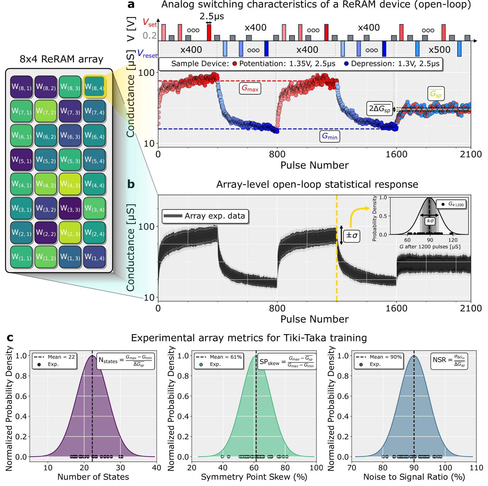
## [Technical Diagram & Charts]: ReRAM Device Characteristics and Array Metrics ### Overview This image is a composite technical figure from a research document, presenting experimental data on Resistive Random-Access Memory (ReRAM) devices. It is divided into three main panels (a, b, c) that collectively characterize the analog switching behavior of a single device, the statistical response of an 8x4 array, and key performance metrics relevant to a training algorithm called "Tiki-Taka." The figure combines a schematic diagram, time-series conductance plots, and statistical distribution histograms. ### Components/Axes **Panel a: Analog switching characteristics of a ReRAM device (open-loop)** * **Left Schematic:** An "8x4 ReRAM array" is depicted as a grid of 32 cells. Each cell is labeled with a weight notation `W(row, column)`, where rows range from 1 to 8 and columns from 1 to 4. Cells are color-coded in shades of purple, green, and teal, likely representing different conductance states or device variations. * **Top Inset (Pulse Sequence):** A timing diagram shows the applied voltage pulse sequence. * **Y-axis:** `V [V]` (Voltage in Volts). Two levels are marked: `V_set` (red, ~0.2V) and `V_reset` (blue, ~0V). * **X-axis:** Time, with pulse durations marked as `2.5µs`. * **Annotations:** Sequences of pulses are grouped with multipliers: `x400`, `x400`, `x400`, `x500`. * **Legend Box:** "Sample Device: • Potentiation: 1.35V, 2.5µs • Depression: 1.3V, 2.5µs". This defines the red and blue pulse conditions. * **Main Plot:** * **Y-axis (Left):** `Conductance [µS]` (microSiemens), on a logarithmic scale from 10 to 100. * **X-axis:** `Pulse Number`, linear scale from 0 to 2100. * **Data Series:** Two distinct series plotted as scatter points. * **Red Circles:** Correspond to "Potentiation" pulses. The trend shows conductance increasing from a low state to a high state. * **Blue Circles:** Correspond to "Depression" pulses. The trend shows conductance decreasing from a high state to a low state. * **Key Annotations:** * `G_max`: A horizontal red dashed line marking the maximum conductance level (~80-90 µS). * `G_min`: A horizontal blue dashed line marking the minimum conductance level (~15-20 µS). * `G_sp`: A horizontal yellow dashed line marking the "Symmetry Point" conductance (~40-50 µS). * `2ΔG_sp`: A vertical double-headed arrow indicating the conductance range around the symmetry point. **Panel b: Array-level open-loop statistical response** * **Main Plot:** * **Y-axis:** `Conductance [µS]`, same logarithmic scale as panel a. * **X-axis:** `Pulse Number`, same scale (0-2100). * **Data Series:** A thick, dark gray shaded band labeled "Array exp. data" in the legend (top-left). This represents the collective response of multiple devices in the array, showing the mean and spread. * **Key Annotations:** * A vertical yellow dashed line at pulse number ~1200. * `±σ`: A vertical double-headed arrow indicating the standard deviation of the conductance distribution at that pulse number. * **Inset Plot (Top Right):** * **Title:** `G after 1200 pulses [µS]` * **Y-axis:** `Probability Density`, from 0.0 to 1.0. * **X-axis:** Conductance `G [µS]`, from 60 to 120. * **Data:** A black bell curve (Gaussian distribution) with a peak around 90 µS. A shaded region under the curve is marked `±σ`. A single black dot is labeled `G_#1200`. **Panel c: Experimental array metrics for Tiki-Taka training** This panel contains three side-by-side histograms. * **Common Y-axis (All three):** `Normalized Probability Density`, from 0.0 to 1.0. * **Left Histogram:** * **X-axis:** `Number of States`, from 10 to 40. * **Data:** Purple shaded distribution with black experimental data points (`Exp.`) along the x-axis. * **Legend:** `--- Mean = 22`. * **Formula Box:** `N_states = (G_max - G_min) / ΔG_sp` * **Middle Histogram:** * **X-axis:** `Symmetry Point Skew (%)`, from 20 to 100. * **Data:** Green shaded distribution with black experimental data points. * **Legend:** `--- Mean = 61%`. * **Formula Box:** `SP_skew = (G_max - G_sp) / (G_max - G_min)` * **Right Histogram:** * **X-axis:** `Noise to Signal Ratio (%)`, from 70 to 110. * **Data:** Blue shaded distribution with black experimental data points. * **Legend:** `--- Mean = 90%`. * **Formula Box:** `NSR = σ_ΔG_sp / ΔG_sp` ### Detailed Analysis **Panel a Analysis:** The single-device characteristic shows clear, analog switching. The conductance increases (potentiates) over the first ~400 pulses, saturating near `G_max`. A subsequent depression phase (~400 pulses) reduces conductance to `G_min`. This cycle repeats. The final phase (starting at pulse 1600) shows a different behavior where conductance oscillates around the symmetry point `G_sp`, with a variation denoted by `2ΔG_sp`. The pulse sequence inset confirms that potentiation and depression are achieved with slightly different voltage amplitudes (1.35V vs. 1.3V). **Panel b Analysis:** The array-level data shows a similar potentiation-depression cycle but as a statistical ensemble. The shaded band indicates device-to-device variability. The inset probability density function confirms that after 1200 pulses, the conductance of devices in the array follows a normal (Gaussian) distribution centered at approximately 90 µS, with a standard deviation (`σ`) of roughly ±10 µS (estimated from the 60-120 µS range). **Panel c Analysis:** The three histograms quantify key metrics for the array: 1. **Number of States (`N_states`):** The distribution is centered at a mean of 22 distinct conductance states. The data points show a spread from about 15 to 30 states. 2. **Symmetry Point Skew (`SP_skew`):** The mean skew is 61%, indicating the symmetry point `G_sp` is not perfectly centered between `G_max` and `G_min`. A value of 50% would be perfectly centered; 61% suggests `G_sp` is closer to `G_max`. 3. **Noise to Signal Ratio (`NSR`):** The mean NSR is 90%, which is very high. This metric (`σ_ΔG_sp / ΔG_sp`) suggests the noise (standard deviation of conductance change around the symmetry point) is nearly as large as the signal (the conductance change itself), indicating significant variability or noise in the device's analog state. ### Key Observations 1. **Analog, Not Binary:** The ReRAM devices exhibit continuous, analog conductance modulation, not just high/low states. 2. **Cyclical Behavior:** Both single-device and array responses show repeatable potentiation and depression cycles. 3. **Device Variability:** Panel b explicitly shows the spread in conductance across the array, which is a critical challenge for analog hardware. 4. **High Noise:** The NSR mean of 90% in panel c is a standout observation, highlighting a major source of error for precise weight storage in neuromorphic computing. 5. **Asymmetry:** The `SP_skew` of 61% indicates an asymmetric switching characteristic, where the midpoint conductance is not equidistant from the extremes. ### Interpretation This figure provides a comprehensive experimental characterization of a ReRAM crossbar array intended for neuromorphic computing, specifically for a training algorithm named "Tiki-Taka." The data moves from the fundamental physics of a single device (panel a) to the collective, statistical behavior of an array (panel b), and finally to derived metrics that directly impact learning performance (panel c). The **core message** is a realistic assessment of the hardware's capabilities and limitations. While the devices successfully demonstrate analog switching—a prerequisite for synaptic weight emulation—the array exhibits substantial device-to-device variability (panel b) and high intrinsic noise (panel c, NSR=90%). The asymmetry in switching (SP_skew=61%) would also complicate symmetric weight updates during training. The "Number of States" (~22) is a practical measure of the effective bit-precision the hardware can support. For a neural network, this translates to the granularity with which synaptic weights can be represented. The combination of limited states, high noise, and asymmetry presents significant challenges for achieving high-accuracy training on this hardware, which the associated research paper likely aims to address with the "Tiki-Taka" algorithm. The figure essentially sets the stage by defining the non-ideal hardware constraints that the algorithm must overcome.

## Chart/Diagram Type: Analog Switching Characteristics of a ReRAM Device (Open-Loop) ### Overview The image presents three interconnected technical visualizations analyzing a ReRAM (Resistive Random-Access Memory) device's behavior. Section **a** shows analog switching characteristics, **b** depicts array-level statistical responses, and **c** summarizes experimental metrics for Tiki-Taka training. --- ### Components/Axes #### Section a: Analog Switching Characteristics - **X-axis**: Pulse Number (0–2100) - **Y-axis**: Conductance [μS] (logarithmic scale: 0–100) - **Legend**: - Red: Potentiation (1.35V, 2.5μs) - Blue: Depression (1.3V, 2.5μs) - **Inset**: Histogram of conductance after 1200 pulses (G₁₂₀₀) with ±σ shading. #### Section b: Array-Level Open-Loop Statistical Response - **X-axis**: Pulse Number (0–2100) - **Y-axis**: Conductance [μS] (logarithmic scale: 0–100) - **Legend**: Array experimental data (black line with ±σ shading). - **Inset**: Histogram of conductance after 1200 pulses (G₁₂₀₀) with ±σ shading. #### Section c: Experimental Array Metrics for Tiki-Taka Training - **Histograms**: 1. **Number of States**: X-axis (0–40), mean = 22. 2. **Symmetry Point Skew (%)**: X-axis (20–110), mean = 61%. 3. **Noise to Signal Ratio (%)**: X-axis (70–110), mean = 90%. - **Formulas**: - N_states = (G_max - G_min) / ΔG_sp - SP_skew = (G_max - G_sp) / G_max - NSR = σΔG_sp / ΔG_sp --- ### Detailed Analysis #### Section a - **Potentiation (Red)**: Conductance increases sharply to ~100 μS at ~800 pulses, then stabilizes. - **Depression (Blue)**: Conductance drops to ~10 μS at ~1600 pulses, then stabilizes. - **Key Labels**: - G_max ≈ 100 μS (potentiation peak). - G_min ≈ 10 μS (depression trough). - ΔG_sp ≈ 90 μS (difference between G_max and G_sp). - G_sp ≈ 10 μS (conductance at symmetry point). #### Section b - **Array Data**: Conductance fluctuates between ~10 μS and ~100 μS, with ±σ shading indicating variability. - **Inset Histogram**: Conductance distribution after 1200 pulses is approximately normal (G₁₂₀₀ ≈ 50 μS, ±σ ≈ ±10 μS). #### Section c - **Number of States**: Bimodal distribution with mean = 22. - **Symmetry Point Skew**: Right-skewed distribution (mean = 61%). - **Noise to Signal Ratio**: Left-skewed distribution (mean = 90%). --- ### Key Observations 1. **Conductance Switching**: Potentiation and depression create distinct conductance states (G_max ≈ 100 μS, G_min ≈ 10 μS). 2. **Statistical Variability**: Shaded regions in **b** indicate device-to-device or batch-to-batch variability. 3. **Training Metrics**: - Tiki-Taka training increases the number of conductance states (mean = 22). - Symmetry point skew (61%) and noise-to-signal ratio (90%) suggest trade-offs between precision and noise. --- ### Interpretation - **ReRAM Behavior**: The device exhibits bistable conductance switching, critical for memory applications. - **Array-Level Variability**: The ±σ shading in **b** highlights manufacturing or operational inconsistencies. - **Tiki-Taka Training**: The metrics in **c** quantify how training affects device performance: - Increased states (N_states) improve memory capacity. - High skew (61%) and noise (90%) may limit reliability. - **Trade-offs**: Optimizing for one metric (e.g., N_states) may degrade others (e.g., NSR). --- **Note**: All values are approximate, derived from visual inspection of axis scales and legend labels. Uncertainties (e.g., ±σ) are inferred from shaded regions and histogram spreads.