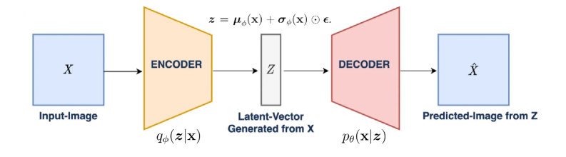
\n ## Diagram: Variational Autoencoder (VAE) Architecture ### Overview The image is a technical schematic diagram illustrating the architecture of a Variational Autoencoder (VAE), a type of generative model in machine learning. It depicts the flow of data from an input image, through an encoding process to a compressed latent representation, and then through a decoding process to generate a predicted output image. The diagram uses colored shapes, arrows, and mathematical notation to represent the model's components and their functions. ### Components/Axes The diagram is organized linearly from left to right, representing the data flow. The components are: 1. **Input Block (Leftmost):** * A light blue square labeled **"X"** in its center. * Below the square, the text **"Input-Image"**. * An arrow points from this block to the next component. 2. **Encoder Block:** * A yellow trapezoid (wider at the input side, narrower at the output) labeled **"ENCODER"** in its center. * Below the trapezoid, the mathematical notation **"\( q_\phi(z|x) \)"**. * An arrow points from this block to the next component. 3. **Latent Vector Block (Center):** * A gray vertical rectangle labeled **"Z"** in its center. * Above the rectangle, the mathematical equation: **"\( z = \mu_\phi(x) + \sigma_\phi(x) \odot \epsilon \)"**. * Below the rectangle, the text **"Latent-Vector Generated from X"**. * An arrow points from this block to the next component. 4. **Decoder Block:** * A pink trapezoid (narrower at the input side, wider at the output) labeled **"DECODER"** in its center. * Below the trapezoid, the mathematical notation **"\( p_\theta(x|z) \)"**. * An arrow points from this block to the final component. 5. **Output Block (Rightmost):** * A light blue square labeled **"\( \hat{X} \)"** (X-hat) in its center. * Below the square, the text **"Predicted-Image from Z"**. ### Detailed Analysis The diagram explicitly defines the probabilistic and generative nature of the VAE: * **Data Flow:** The process is unidirectional: `Input-Image (X) -> ENCODER -> Latent-Vector (Z) -> DECODER -> Predicted-Image (\( \hat{X} \))`. * **Encoder Function:** The encoder, parameterized by \(\phi\), is represented by the distribution \( q_\phi(z|x) \). It maps the high-dimensional input `X` to a probability distribution in the lower-dimensional latent space `Z`. * **Latent Sampling:** The equation \( z = \mu_\phi(x) + \sigma_\phi(x) \odot \epsilon \) describes the **reparameterization trick**. It shows that a latent vector `z` is sampled by taking the mean (\(\mu_\phi(x)\)) and standard deviation (\(\sigma_\phi(x)\)) predicted by the encoder for input `x`, and adding noise scaled by \(\sigma_\phi(x)\). The symbol \(\odot\) denotes element-wise multiplication, and \(\epsilon\) represents random noise (typically from a standard normal distribution). * **Decoder Function:** The decoder, parameterized by \(\theta\), is represented by the distribution \( p_\theta(x|z) \). It attempts to reconstruct or generate a plausible data point `x` (the predicted image \(\hat{X}\)) from the sampled latent vector `z`. * **Visual Metaphor:** The trapezoidal shapes are a common visual metaphor: the encoder "compresses" the data (wide to narrow), and the decoder "reconstructs" or "expands" it (narrow to wide). ### Key Observations 1. **Color Coding:** Components are consistently color-coded: blue for data (input/output), yellow for the encoder, gray for the latent space, and pink for the decoder. 2. **Mathematical Precision:** The diagram includes the core mathematical formulations that define a VAE, distinguishing it from a standard autoencoder. The presence of the distribution notations \( q_\phi(z|x) \) and \( p_\theta(x|z) \), along with the reparameterization equation, is critical. 3. **Label Clarity:** Every component and connection is explicitly labeled with both a descriptive name (e.g., "Input-Image") and its mathematical symbol (e.g., "X"). 4. **Spatial Grounding:** The legend/labels are placed directly adjacent to their corresponding components (below the boxes/trapezoids, above the latent vector), ensuring unambiguous association. ### Interpretation This diagram is a foundational representation of a Variational Autoencoder. It visually explains the model's two-stage generative process: 1. **Inference (Encoding):** The model learns to map complex input data (like images) to a structured, continuous latent space. The encoder doesn't produce a single code but parameters of a distribution (\(\mu\) and \(\sigma\)), introducing stochasticity which is key for generation. 2. **Generation (Decoding):** By sampling a point `z` from this learned latent space and passing it through the decoder, the model can generate new, synthetic data instances (\(\hat{X}\)) that resemble the original training data. The **reparameterization trick** (the equation above Z) is highlighted as a crucial technical innovation. It allows for backpropagation through the stochastic sampling node, making the entire network trainable via gradient descent. The diagram's purpose is pedagogical and technical. It abstracts away the specific neural network layers (e.g., convolutional, fully connected) to focus on the high-level architecture and probabilistic framework. It communicates that a VAE is not merely a compression tool but a **probabilistic generative model** that learns the underlying distribution of the data, enabling tasks like image generation, interpolation in latent space, and denoising. The clear separation of \(\phi\) (encoder parameters) and \(\theta\) (decoder parameters) underscores that these are two distinct, jointly trained neural networks.