## Diagram: Autoencoder Architecture
### Overview
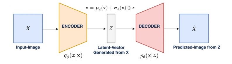
The diagram illustrates the structure of an autoencoder, a type of neural network used for unsupervised learning. It shows the flow of data from an input image (X) through an encoder to a latent vector (Z), then through a decoder to reconstruct a predicted image (Ẋ). Key equations and probabilistic relationships are annotated.
### Components/Axes
1. **Input-Image**: Labeled as **X** (blue box).
2. **Encoder**:
- Outputs two components:
- **qφ(z|x)**: Probability distribution of latent vector Z given input X (orange trapezoid).
- **z = μφ(x) + σφ(x) ⊙ ε**: Latent vector Z decomposed into mean (μφ(x)), standard deviation (σφ(x)), and noise (ε) via element-wise multiplication (⊙).
3. **Latent-Vector**:
- Labeled as **Z** (gray rectangle).
- Described as "Latent-Vector Generated from X."
4. **Decoder**:
- Outputs **pθ(x|z)**: Probability distribution of reconstructed input X given latent vector Z (pink trapezoid).
5. **Predicted-Image**: Labeled as **Ẋ** (blue box).
### Detailed Analysis
- **Encoder Function**:
- Maps input image X to a latent representation Z.
- Z is parameterized by a mean (μφ(x)) and standard deviation (σφ(x)), with noise (ε) added via element-wise multiplication.
- The distribution **qφ(z|x)** represents the encoder's learned mapping.
- **Decoder Function**:
- Reconstructs the input image from Z using **pθ(x|z)**, a probability distribution over X conditioned on Z.
- The decoder learns to invert the encoder's mapping.
- **Equations**:
- **z = μφ(x) + σφ(x) ⊙ ε**:
- μφ(x): Mean of the latent distribution.
- σφ(x): Standard deviation of the latent distribution.
- ε: Noise vector (element-wise multiplied with σφ(x)).
- **pθ(x|z)**: Decoder's output distribution, parameterized by θ.
### Key Observations
1. **Probabilistic Framework**: The autoencoder uses probabilistic distributions (qφ and pθ) to model uncertainty in latent representations and reconstructions.
2. **Latent Space**: Z acts as a compressed, abstract representation of X, capturing essential features.
3. **Noise Injection**: The term **⊙ ε** introduces stochasticity, enabling the model to generalize beyond exact reconstructions.
4. **Directionality**: Data flows unidirectionally from X → Z → Ẋ, with no feedback loops.
### Interpretation
This diagram represents a **Variational Autoencoder (VAE)**, a generative model that learns to:
- **Compress** input data into a latent space (Z) via the encoder.
- **Reconstruct** data from Z via the decoder, while adhering to a probabilistic framework.
- The equations highlight the VAE's reliance on variational inference, where the encoder approximates the true data distribution and the decoder generates samples from the latent space.
The architecture is foundational for tasks like image generation, denoising, and feature extraction, with the latent vector Z serving as a compact, meaningful representation of the input data.