## Comparison of Neural Network Architectures: MLP vs KAN
### Overview
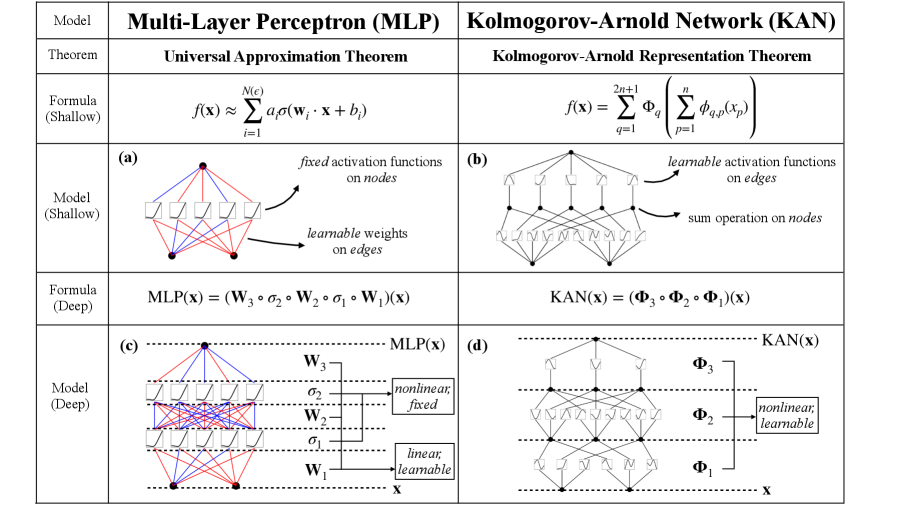
The image compares two neural network architectures: Multi-Layer Perceptron (MLP) and Kolmogorov-Arnold Network (KAN). It includes theoretical foundations, mathematical formulations, and visual diagrams for both shallow and deep implementations.
### Components/Axes
1. **Theoretical Foundations**:
- MLP: Universal Approximation Theorem
- KAN: Kolmogorov-Arnold Representation Theorem
2. **Formulas**:
- **MLP (Shallow)**:
`f(x) ≈ Σᴵ=1^N(C) aᵢσ(wᵢ·x + bᵢ)`
(Sum of weighted inputs with fixed activation functions and learnable weights/biases)
- **KAN (Shallow)**:
`f(x) = Σᴵ=1^(2n+1) Φᵢ(Σₚ=1^n φₚ,ₚ(xₚ))`
(Sum of compositional functions with learnable activation functions)
3. **Model Diagrams**:
- **MLP (Shallow)**: Diagram (a) shows fixed activation functions on nodes and learnable weights on edges.
- **KAN (Shallow)**: Diagram (b) shows learnable activation functions on edges and sum operations on nodes.
- **MLP (Deep)**: Diagram (c) shows layered architecture with fixed and learnable weights.
- **KAN (Deep)**: Diagram (d) shows layered architecture with fixed and learnable activation functions.
4. **Formulas (Deep)**:
- **MLP**: `MLP(x) = (W₃·σ₂·W₂·σ₁·W₁)(x)`
(Composition of weight matrices and fixed activation functions)
- **KAN**: `KAN(x) = (Φ₃·Φ₂·Φ₁)(x)`
(Composition of learnable activation functions)
### Detailed Analysis
- **MLP Structure**:
- Shallow: Single hidden layer with fixed activation functions (σ) and learnable weights (W) and biases (b).
- Deep: Multi-layer architecture with alternating learnable weights (W₁, W₂, W₃) and fixed activation functions (σ₁, σ₂).
- **KAN Structure**:
- Shallow: Single hidden layer with learnable activation functions (φ) and fixed sum operations (Σ).
- Deep: Multi-layer architecture with alternating learnable activation functions (Φ₁, Φ₂, Φ₃) and fixed sum operations.
### Key Observations
1. **Learnable Parameters**:
- MLP: Weights and biases are learnable; activation functions are fixed.
- KAN: Activation functions are learnable; sum operations are fixed.
2. **Compositional Differences**:
- MLP uses matrix multiplications (W·σ) between layers.
- KAN uses function composition (Φ·Φ) between layers.
3. **Theoretical Guarantees**:
- MLP's universal approximation relies on fixed activation functions with sufficient width.
- KAN's representation theorem enables efficient function decomposition through learnable activation functions.
### Interpretation
The comparison reveals fundamental architectural differences:
1. **Function Representation**:
- MLP approximates functions through linear combinations of fixed nonlinearities.
- KAN decomposes functions into compositions of learnable activation functions, potentially enabling more efficient representations for certain classes of functions.
2. **Training Dynamics**:
- MLP trains weights/biases while keeping activation functions fixed.
- KAN trains activation functions while keeping sum operations fixed, which may lead to different optimization landscapes.
3. **Theoretical Implications**:
- The Kolmogorov-Arnold theorem provides a more flexible function decomposition framework compared to the universal approximation theorem's reliance on fixed activation functions.
4. **Practical Considerations**:
- KAN's learnable activation functions might offer better expressivity for complex function interactions.
- MLP's fixed activation functions could lead to more stable training but potentially limited representational power.
This analysis suggests that KAN's architecture may be particularly advantageous for problems requiring complex function decomposition, while MLP remains a robust choice for standard feedforward tasks with well-understood activation functions.