## Composite Figure: Quantum Computing and Machine Learning
### Overview
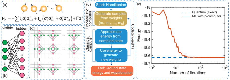
The image is a composite figure illustrating a quantum computing approach combined with machine learning. It includes a schematic of a quantum system, a neural network representation, a computational flow diagram, and a convergence plot comparing the energy of a quantum system calculated exactly versus using a machine learning approach with a probabilistic computer.
### Components/Axes
* **(a) Quantum System Schematic:**
* A series of spheres, presumably representing atoms or qubits, with arrows indicating spin directions.
* Equation: H\_Q = - Σ J\_z σ^z\_i σ^z\_{i+1} + J\_{xy} (σ^x\_i σ^x\_{i+1} + σ^y\_i σ^y\_{i+1}) + Γ σ^x\_i
* **(b) Neural Network Representation:**
* "visible" layer: A column of green circles on the left.
* "hidden" layer: A column of pink circles on the right.
* Lines connecting each node in the visible layer to each node in the hidden layer.
* **(c) Lattice Structure:**
* A grid-like structure with repeating units. Each unit contains green and pink circles connected by lines.
* **(d) Computational Flow Diagram:**
* Divided into "Probabilistic computer" and "Classical computer" sections.
* Flow:
1. Start: Hamiltonian (Blue rectangle)
2. Generate samples from weights {m1, m2, ..., mN} (Gold rectangle)
3. Approximate energy from sampled state (Blue rectangle)
4. Use energy to generate new weights (Blue rectangle)
5. Update weights (Arrow pointing back to step 2)
6. End: Ground state energy and wavefunction (Orange rectangle)
* **(e) Convergence Plot:**
* X-axis: Number of iterations (Logarithmic scale from 10^0 to 10^31)
* Y-axis: Energy (Linear scale from -18.7 to -18)
* Legend (Top-right):
* Blue dashed line: Quantum (exact)
* Red solid line: ML with p-computer
### Detailed Analysis
* **(a) Quantum System:**
* The equation represents a Hamiltonian, likely for an Ising-type model with transverse field.
* J\_z and J\_{xy} are coupling constants.
* σ^z, σ^x, and σ^y are Pauli matrices.
* Γ represents the transverse field strength.
* **(b) Neural Network:**
* The network has a visible layer with approximately 5 nodes and a hidden layer with approximately 5 nodes.
* The "..." indicates that the layers can have more nodes.
* **(c) Lattice Structure:**
* The lattice appears to be a 2D grid.
* Each repeating unit has a diamond shape formed by the connections between green and pink circles.
* **(d) Computational Flow:**
* The algorithm iteratively refines the weights of a probabilistic computer using a classical computer to approximate the ground state energy.
* **(e) Convergence Plot:**
* The blue dashed line (Quantum (exact)) is a horizontal line at approximately -18.65.
* The red solid line (ML with p-computer) starts at approximately -18.0 and rapidly decreases, converging to approximately -18.65 after about 10 iterations.
* The x-axis is a log scale.
### Key Observations
* The machine learning approach converges to the exact quantum result after a relatively small number of iterations.
* The initial energy estimate from the machine learning approach is significantly higher than the exact quantum energy.
* The algorithm effectively minimizes the energy by adjusting the weights of the probabilistic computer.
### Interpretation
The figure demonstrates a hybrid quantum-classical approach to solving a quantum problem. The machine learning algorithm, implemented on a probabilistic computer, learns to approximate the ground state energy of a quantum system. The convergence plot shows that the machine learning approach can accurately reproduce the exact quantum result, suggesting that this hybrid approach could be a powerful tool for studying complex quantum systems. The neural network and lattice structure likely represent the underlying architecture used in the machine learning model. The computational flow diagram provides a clear overview of the algorithm's steps.