## Diagram: Variational Quantum Eigensolver (VQE) Workflow
### Overview
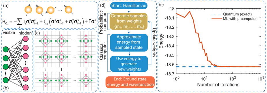
The image depicts a workflow diagram illustrating the Variational Quantum Eigensolver (VQE) algorithm, alongside a representation of the Hamiltonian and a performance comparison chart. The diagram outlines the iterative process of using a probabilistic computer (quantum computer) to generate samples, a classical computer to approximate energy, and update weights to converge towards the ground state energy and wavefunction.
### Components/Axes
The image is divided into four main sections: (a) Hamiltonian representation, (b) Neural Network representation, (c) Quantum-Classical interaction, and (e) Performance comparison chart.
* **(a) Hamiltonian:** Displays the equation for the Hamiltonian: `H₀ = Σᵢ σₓⁱ + Σᵢ<ⱼ Jₓᵣ (σₓⁱσₓᵣ + σᵧⁱσᵧᵣ) + Γσ₂`.
* **(b) Neural Network:** Shows a multi-layered neural network with visible and hidden layers.
* **(c) Quantum-Classical Interaction:** Illustrates the interaction between a probabilistic (quantum) computer and a classical computer.
* **(e) Performance Chart:**
* **X-axis:** Number of iterations (logarithmic scale, from 10⁰ to 10³).
* **Y-axis:** Energy (ranging from approximately -18.1 to -18.7).
* **Data Series:**
* "Quantum (exact)" - represented by a dashed blue line.
* "ML with p-computer" - represented by a solid orange line.
### Detailed Analysis or Content Details
**(a) Hamiltonian:** The equation represents a spin Hamiltonian, likely used to describe a physical system. The symbols represent Pauli matrices (σₓ, σᵧ, σ₂) and coupling constants (Jₓᵣ, Γ).
**(b) Neural Network:** The neural network has 7 visible nodes (green) and 5 hidden nodes (red). The connections between nodes are not explicitly labeled with weights.
**(c) Quantum-Classical Interaction:** This section details the VQE algorithm steps:
1. **Start:** Hamiltonian is defined.
2. **Probabilistic Computer:** Generate samples from weights (m₁, m₂, ..., mₙ).
3. **Classical Computer:** Approximate energy from sampled state.
4. **Classical Computer:** Use energy to generate new weights.
5. **End:** Ground state energy and wavefunction.
**(e) Performance Chart:**
* **Quantum (exact):** The blue dashed line starts at approximately -18.12 and remains relatively constant, fluctuating slightly around -18.11 to -18.13 across the entire range of iterations.
* **ML with p-computer:** The orange solid line starts at approximately -18.08 and exhibits a steep downward trend initially. It reaches approximately -18.65 at around 10¹ iterations. After this point, the slope decreases, and the line continues to descend, approaching -18.12 at 10³ iterations.
### Key Observations
* The ML with p-computer line demonstrates a clear convergence towards the energy value of the Quantum (exact) line.
* The initial convergence of the ML method is rapid, but slows down as it approaches the exact solution.
* The Quantum (exact) line remains stable, indicating the true ground state energy.
* The diagram visually represents the iterative nature of the VQE algorithm, where the classical computer refines the weights based on the energy estimates from the quantum computer.
### Interpretation
The diagram illustrates the core principles of the Variational Quantum Eigensolver (VQE) algorithm. The algorithm leverages a hybrid quantum-classical approach to find the ground state energy of a given Hamiltonian. The quantum computer generates samples, which are then used by a classical computer to estimate the energy. This energy estimate is used to update the parameters of a variational ansatz (represented by the neural network in section (b)), iteratively refining the solution.
The performance chart (e) demonstrates the effectiveness of this approach. The ML with p-computer line's convergence towards the Quantum (exact) line indicates that the algorithm is successfully finding the ground state energy. The initial rapid convergence suggests that the algorithm quickly learns the essential features of the energy landscape, while the slower convergence at later stages indicates that it is fine-tuning the solution to achieve higher accuracy.
The Hamiltonian equation (a) provides the mathematical foundation for the problem being solved, while the neural network (b) represents the variational ansatz used to approximate the ground state wavefunction. The diagram as a whole provides a comprehensive overview of the VQE algorithm, highlighting its key components and workflow. The use of a logarithmic scale on the x-axis of the performance chart emphasizes the iterative nature of the algorithm and the gradual improvement in accuracy over time.