## [Composite Diagram]: Hybrid Quantum-Classical Algorithm for Ground State Estimation
### Overview
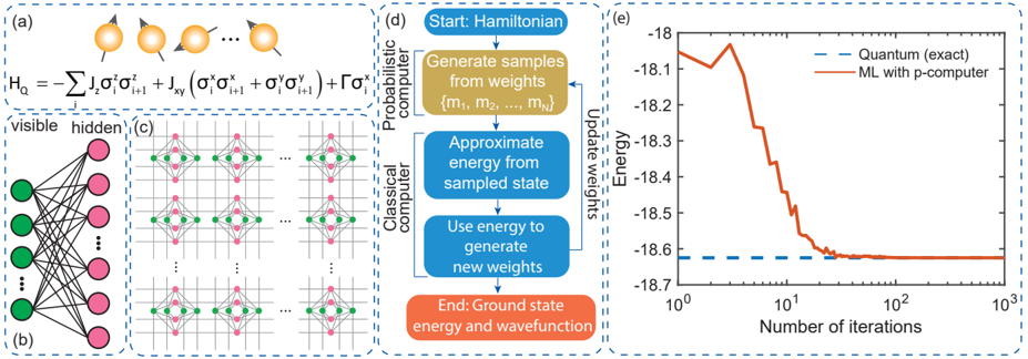
The image is a composite of five components (a–e) illustrating a **hybrid quantum-classical algorithm** (e.g., Variational Quantum Eigensolver, VQE) for estimating the ground state of a quantum Hamiltonian. It combines quantum mechanics, graphical models, lattice structures, a computational flowchart, and a convergence plot.
### Components/Axes
#### (a) Quantum Hamiltonian & Spin Representation
- **Equation**: \( \boldsymbol{H_Q = -\sum J_i \sigma_i^z \sigma_{i+1}^z + J_{xy} (\sigma_i^x \sigma_{i+1}^x + \sigma_i^y \sigma_{i+1}^y) + \Gamma \sigma_i^x} \)
(Describes a quantum system with Ising (\( \sigma^z \sigma^z \)), XY (\( \sigma^x \sigma^x + \sigma^y \sigma^y \)), and transverse field (\( \Gamma \sigma^x \)) interactions, typical of spin models like the transverse-field Ising model with XY couplings.)
- **Visual**: Orange circles with arrows (spins/qubits) in a chain, representing a 1D or quasi-1D quantum system.
#### (b) Graphical Model (Visible-Hidden Layers)
- **Structure**: Green nodes (labeled “visible”) and pink nodes (labeled “hidden”) connected by lines (edges).
- **Interpretation**: A neural network or Restricted Boltzmann Machine (RBM)-like ansatz, where hidden nodes encode auxiliary degrees of freedom to approximate the quantum state.
#### (c) Lattice Structure
- **Structure**: A 2D grid of green (visible) and pink (hidden) nodes, likely a square lattice (e.g., for a 2D spin system).
- **Interpretation**: Represents the spatial structure of the quantum system (e.g., a lattice of spins/qubits with nearest-neighbor interactions).
#### (d) Computational Flowchart
- **Sections**:
- *Probabilistic computer* (blue boxes): Quantum sampling to estimate energy.
- *Classical computer* (orange boxes): Classical optimization to update weights.
- **Steps** (with arrows):
1. Start: Hamiltonian (\( H_Q \))
2. Generate samples from weights \( \{m_1, m_2, ..., m_N\} \)
3. Approximate energy from sampled state
4. Use energy to generate new weights
5. Update weights
6. End: Ground state energy and wavefunction
#### (e) Convergence Plot
- **Axes**:
- *X-axis*: “Number of iterations” (logarithmic scale: \( 10^0, 10^1, 10^2, 10^3 \))
- *Y-axis*: “Energy” (linear scale: \( -18.7 \) to \( -18 \))
- **Lines**:
- *Blue dashed*: “Quantum (exact)” (constant energy, ~\( -18.65 \), representing the exact ground state energy).
- *Red solid*: “ML with p-computer” (decreasing energy, converging to the blue line as iterations increase).
### Detailed Analysis
#### (a) Hamiltonian
The equation describes a quantum system with:
- Ising interactions (\( -\sum J_i \sigma_i^z \sigma_{i+1}^z \)): Aligns spins along the \( z \)-axis.
- XY interactions (\( J_{xy} (\sigma_i^x \sigma_{i+1}^x + \sigma_i^y \sigma_{i+1}^y) \)): Allows spin flips in the \( x \)-\( y \) plane.
- Transverse field (\( \Gamma \sigma_i^x \)): Induces quantum fluctuations.
#### (b) Graphical Model
The visible (green) and hidden (pink) nodes suggest a **variational ansatz** (e.g., a neural network or RBM) to approximate the quantum state. Hidden nodes capture correlations not directly visible in the physical system.
#### (c) Lattice
The 2D grid implies a **spatially extended quantum system** (e.g., a square lattice of spins), where green/pink nodes may represent different spin states or layers (e.g., a bipartite lattice).
#### (d) Flowchart
The iterative process (quantum sampling → classical optimization) is a hallmark of **hybrid quantum-classical algorithms** (e.g., VQE). Quantum sampling (probabilistic computer) estimates energy, while classical ML updates weights to minimize energy, converging to the ground state.
#### (e) Convergence Plot
- The *red line* (ML with p-computer) starts at ~\( -18.1 \), decreases rapidly, and approaches the *blue dashed line* (exact quantum energy) as iterations increase (from \( 10^0 \) to \( 10^3 \)).
- The *blue line* is horizontal, confirming the exact ground state energy is constant.
### Key Observations
- The hybrid approach (quantum sampling + classical ML) **converges to the exact quantum ground state energy**.
- The graphical model (b) and lattice (c) provide a **structured ansatz** to capture spatial correlations in the quantum state.
- The flowchart (d) emphasizes **iterative feedback** between quantum sampling and classical optimization.
### Interpretation
This image illustrates a hybrid quantum-classical algorithm for finding the ground state of a quantum Hamiltonian (a). The graphical model (b) and lattice (c) define a variational ansatz to represent the quantum state. The flowchart (d) outlines the iterative process: quantum sampling (probabilistic computer) estimates energy, while classical ML updates weights to minimize energy. The convergence plot (e) shows the ML approach (with p-computer) approximates the exact quantum energy, demonstrating the effectiveness of the hybrid method.
This is critical for quantum computing tasks where exact quantum simulation is infeasible, and classical ML aids in optimizing variational parameters. The algorithm balances quantum sampling (to capture quantum correlations) and classical optimization (to efficiently update weights), enabling accurate ground state estimation for complex quantum systems.
(Note: All text is in English; no non-English text is present.)