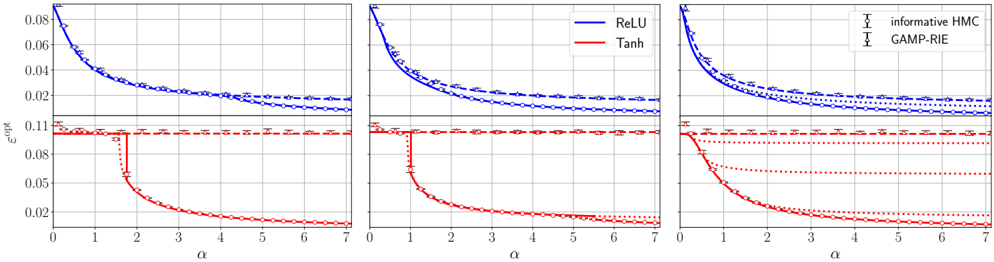
## Chart: Comparison of ReLU and Tanh Activation Functions with Different Methods ### Overview The image presents three line charts comparing the performance of ReLU (Rectified Linear Unit) and Tanh (Hyperbolic Tangent) activation functions under different conditions. The charts share the same x-axis, labeled "α", and y-axis, labeled "εopt". Each chart represents a different method (informative HMC and GAMP-RIE). The performance is evaluated based on the error rate, with lower values indicating better performance. ### Components/Axes * **X-axis:** "α" - Ranges from 0 to 7, with tick marks at every integer value. * **Y-axis:** "εopt" - Ranges from 0.02 to 0.08 in the top half of the chart and 0.02 to 0.11 in the bottom half of the chart. * **Legend (Top-Right):** * Blue Line: ReLU * Red Line: Tanh * Informative HMC: Error bars with circles * GAMP-RIE: Error bars with horizontal bars ### Detailed Analysis Each of the three charts displays two sets of curves: one for ReLU (blue) and one for Tanh (red). Each set contains three curves: a solid line, a dashed line, and a dotted line. The solid and dashed lines have error bars. **Chart 1 (Left):** * **ReLU (Blue):** The solid blue line with circular error bars (informative HMC) starts at approximately 0.08 at α=0 and decreases to approximately 0.02 at α=7. The dashed blue line with horizontal error bars (GAMP-RIE) starts at approximately 0.07 at α=0 and decreases to approximately 0.02 at α=7. The dotted blue line starts at approximately 0.06 at α=0 and decreases to approximately 0.02 at α=7. * **Tanh (Red):** The solid red line with circular error bars (informative HMC) starts at approximately 0.11 at α=0, drops sharply to approximately 0.05 at α=1.5, and then decreases to approximately 0.02 at α=7. The dashed red line with horizontal error bars (GAMP-RIE) remains constant at approximately 0.105 from α=0 to α=7. The dotted red line starts at approximately 0.10 at α=0, drops sharply to approximately 0.05 at α=1.5, and then decreases to approximately 0.02 at α=7. **Chart 2 (Middle):** * **ReLU (Blue):** The solid blue line with circular error bars (informative HMC) starts at approximately 0.08 at α=0 and decreases to approximately 0.02 at α=7. The dashed blue line with horizontal error bars (GAMP-RIE) starts at approximately 0.07 at α=0 and decreases to approximately 0.02 at α=7. The dotted blue line starts at approximately 0.06 at α=0 and decreases to approximately 0.02 at α=7. * **Tanh (Red):** The solid red line with circular error bars (informative HMC) starts at approximately 0.11 at α=0, drops sharply to approximately 0.05 at α=1.5, and then decreases to approximately 0.02 at α=7. The dashed red line with horizontal error bars (GAMP-RIE) remains constant at approximately 0.105 from α=0 to α=7. The dotted red line starts at approximately 0.10 at α=0, drops sharply to approximately 0.05 at α=1.5, and then decreases to approximately 0.02 at α=7. **Chart 3 (Right):** * **ReLU (Blue):** The solid blue line with circular error bars (informative HMC) starts at approximately 0.08 at α=0 and decreases to approximately 0.02 at α=7. The dashed blue line with horizontal error bars (GAMP-RIE) starts at approximately 0.07 at α=0 and decreases to approximately 0.02 at α=7. The dotted blue line starts at approximately 0.06 at α=0 and decreases to approximately 0.02 at α=7. * **Tanh (Red):** The solid red line with circular error bars (informative HMC) starts at approximately 0.11 at α=0, drops sharply to approximately 0.05 at α=1.5, and then decreases to approximately 0.02 at α=7. The dashed red line with horizontal error bars (GAMP-RIE) remains constant at approximately 0.105 from α=0 to α=7. The dotted red line starts at approximately 0.10 at α=0, drops sharply to approximately 0.05 at α=1.5, and then decreases to approximately 0.02 at α=7. ### Key Observations * **ReLU Performance:** The ReLU activation function consistently shows a decreasing error rate as α increases across all three charts. * **Tanh Performance:** The Tanh activation function exhibits a sharp drop in error rate around α=1.5 when using the solid line with circular error bars (informative HMC) and the dotted line. The dashed line with horizontal error bars (GAMP-RIE) remains relatively constant. * **Error Bar Placement:** The error bars are placed vertically on the solid and dashed lines. * **Chart Similarity:** The three charts are nearly identical. ### Interpretation The charts suggest that the ReLU activation function generally performs better than the Tanh activation function, especially at lower values of α. The sharp drop in error rate for Tanh around α=1.5 indicates a critical point where the function's behavior changes significantly. The consistent performance of ReLU across different values of α suggests it might be a more stable choice in these scenarios. The dashed line with horizontal error bars (GAMP-RIE) for Tanh shows a constant error rate, indicating that this method might not be as effective for the Tanh activation function. The similarity of the three charts suggests that the underlying conditions being varied between the charts have little impact on the relative performance of ReLU and Tanh.

## Chart Type: Multi-panel Line Graphs with Phase Transitions ### Overview This image contains three side-by-side panels, each displaying a comparison of two activation functions, **ReLU** (blue lines) and **Tanh** (red lines), across a range of a parameter $\alpha$. Each panel is vertically split into two sub-plots: the top sub-plot focuses on ReLU performance, and the bottom sub-plot focuses on Tanh performance. The charts compare theoretical predictions (lines) with experimental data points from two methods: **informative HMC** and **GAMP-RIE**. ### Components/Axes * **X-axis (all panels):** Labeled $\alpha$, ranging from $0$ to $7$ with major ticks at every integer. * **Y-axis (Top sub-plots):** Labeled $\varepsilon^{opt}$. Scale ranges from approximately $0.01$ to $0.09$, with labeled ticks at $0.02, 0.04, 0.06, 0.08$. * **Y-axis (Bottom sub-plots):** Labeled $\varepsilon^{opt}$. Scale ranges from approximately $0.01$ to $0.11$, with labeled ticks at $0.02, 0.05, 0.08, 0.11$. * **Legends:** * **Middle Panel (Top-Right):** Identifies line colors. * **Blue solid line:** ReLU * **Red solid line:** Tanh * **Right Panel (Top-Right):** Identifies markers and error bars. * **Open Circle ($\circ$) with error bars:** informative HMC * **Open Triangle ($\triangle$) with error bars:** GAMP-RIE * **Line Styles:** * **Solid lines:** Primary theoretical prediction. * **Dashed/Dotted lines:** Secondary theoretical branches or alternative states. --- ### Detailed Analysis The three panels represent different experimental conditions (likely varying signal-to-noise ratios or prior strengths), ordered from left to right. #### 1. Left Panel * **ReLU (Blue, Top):** The error $\varepsilon^{opt}$ starts high ($>0.08$) at $\alpha=0$ and decays smoothly. A dashed line branches upward from the solid line around $\alpha \approx 4.5$. Experimental markers (circles and triangles) closely follow the solid line, reaching $\approx 0.015$ at $\alpha=7$. * **Tanh (Red, Bottom):** The error remains flat at $\approx 0.10$ until a critical point at $\alpha \approx 1.8$. At this point, the solid line drops sharply to $\approx 0.05$ and then decays gradually to $\approx 0.01$. A dashed line continues the flat plateau at $0.10$ for all $\alpha$. Experimental markers follow the sharp drop accurately. #### 2. Middle Panel * **ReLU (Blue, Top):** Similar decay to the left panel, but the branching of the dashed line occurs much earlier, around $\alpha \approx 1.0$. The error at $\alpha=7$ is lower, $\approx 0.01$. * **Tanh (Red, Bottom):** The sharp transition (drop in error) occurs earlier than in the first panel, at $\alpha \approx 1.0$. After the drop, the error decays to $\approx 0.01$ at $\alpha=7$. A dotted line branches off and stays at a higher error level ($\approx 0.015$) for $\alpha > 5.5$. #### 3. Right Panel * **ReLU (Blue, Top):** The error decays even more rapidly. Multiple dotted/dashed lines are visible, branching off at various low $\alpha$ values. The final error at $\alpha=7$ is the lowest of the three panels, $\approx 0.005$. * **Tanh (Red, Bottom):** The transition is very early, occurring at $\alpha \approx 0.3$. There are multiple dotted lines representing metastable states at higher error levels (around $0.09, 0.06, 0.02$). The main solid line and experimental points drop to the lowest error state quickly. --- ### Key Observations * **Phase Transitions:** The Tanh (red) curves exhibit a "hard" phase transition characterized by a sudden, discontinuous drop in error at a critical $\alpha_c$. * **Algorithmic Convergence:** Both **informative HMC** (circles) and **GAMP-RIE** (triangles) show excellent agreement with the theoretical solid lines, successfully "jumping" the gap during phase transitions. * **Branching:** The presence of dashed and dotted lines suggests the existence of multiple fixed points or solutions in the underlying mathematical model (likely a Mean Field theory or Replica analysis), where the solid line represents the global minimum (optimal error). * **Trend across panels:** Moving from left to right, the critical $\alpha$ for the Tanh transition decreases, and the overall achievable error for both models decreases, indicating an increasingly "easier" inference task. --- ### Interpretation The data demonstrates the **learning dynamics of high-dimensional generalized linear models**. * **$\alpha$** likely represents the sampling ratio (number of samples divided by dimensions). As more data is provided (increasing $\alpha$), the error $\varepsilon^{opt}$ decreases. * The **ReLU** model shows a "soft" learning curve where information is gained continuously. * The **Tanh** model exhibits a "computational gap" or "hard" learning regime. Below a certain threshold of data ($\alpha_c$), the model cannot learn better than a random guess (the plateau). Once the threshold is crossed, it undergoes a rapid transition to a high-accuracy state. * The fact that **GAMP-RIE** (an approximate message passing algorithm) and **HMC** (Hamiltonian Monte Carlo) both track the optimal theoretical line suggests that these algorithms are efficient enough to find the global minimum even in the presence of the sharp transitions shown in the Tanh case. * The different panels likely show the effect of increasing the **Signal-to-Noise Ratio (SNR)**. Higher SNR (right panel) makes the transition happen with less data and results in lower final error.

\n ## Chart: Optimal Error Rate vs. Alpha for Different Activation Functions and Inference Methods ### Overview This image presents three line charts, arranged horizontally, displaying the relationship between the optimal error rate (ε_opt) and the alpha (α) parameter. Each chart compares the performance of two activation functions, ReLU and Tanh, under two different inference methods, Informative HMC and GAMP-RIE. The charts share identical axes and scales, allowing for direct comparison across the three panels. ### Components/Axes * **X-axis:** α (Alpha) - Ranging from 0 to 7, with tick marks at integer values. * **Y-axis:** ε_opt (Optimal Error Rate) - Ranging from 0 to 0.08, with tick marks at 0.02 intervals. * **Lines:** * ReLU (Blue) - Represents the optimal error rate for the ReLU activation function. * Tanh (Red) - Represents the optimal error rate for the Tanh activation function. * **Error Bars:** * Informative HMC (Light Blue) - Error bars representing the uncertainty associated with the Informative HMC inference method. * GAMP-RIE (Light Red) - Error bars representing the uncertainty associated with the GAMP-RIE inference method. * **Legend:** Located in the top-right corner, clearly labeling each line and error bar. ### Detailed Analysis or Content Details **Chart 1 (Left):** * **ReLU (Blue):** The line slopes downward from approximately 0.07 at α = 0 to approximately 0.018 at α = 7. The error bars are relatively small, indicating low uncertainty. * α = 0: ε_opt ≈ 0.07 * α = 1: ε_opt ≈ 0.055 * α = 2: ε_opt ≈ 0.04 * α = 3: ε_opt ≈ 0.03 * α = 4: ε_opt ≈ 0.025 * α = 5: ε_opt ≈ 0.022 * α = 6: ε_opt ≈ 0.02 * α = 7: ε_opt ≈ 0.018 * **Tanh (Red):** The line slopes downward more steeply than ReLU, starting at approximately 0.09 at α = 0 and reaching approximately 0.008 at α = 7. The error bars are also relatively small. * α = 0: ε_opt ≈ 0.09 * α = 1: ε_opt ≈ 0.06 * α = 2: ε_opt ≈ 0.035 * α = 3: ε_opt ≈ 0.02 * α = 4: ε_opt ≈ 0.012 * α = 5: ε_opt ≈ 0.009 * α = 6: ε_opt ≈ 0.0085 * α = 7: ε_opt ≈ 0.008 **Chart 2 (Center):** * **ReLU (Blue):** Similar trend to Chart 1, starting at approximately 0.07 and decreasing to approximately 0.018 at α = 7. Error bars are comparable to Chart 1. * α = 0: ε_opt ≈ 0.07 * α = 1: ε_opt ≈ 0.055 * α = 2: ε_opt ≈ 0.04 * α = 3: ε_opt ≈ 0.03 * α = 4: ε_opt ≈ 0.025 * α = 5: ε_opt ≈ 0.022 * α = 6: ε_opt ≈ 0.02 * α = 7: ε_opt ≈ 0.018 * **Tanh (Red):** Similar trend to Chart 1, starting at approximately 0.09 and decreasing to approximately 0.008 at α = 7. Error bars are comparable to Chart 1. * α = 0: ε_opt ≈ 0.09 * α = 1: ε_opt ≈ 0.06 * α = 2: ε_opt ≈ 0.035 * α = 3: ε_opt ≈ 0.02 * α = 4: ε_opt ≈ 0.012 * α = 5: ε_opt ≈ 0.009 * α = 6: ε_opt ≈ 0.0085 * α = 7: ε_opt ≈ 0.008 **Chart 3 (Right):** * **ReLU (Blue):** Similar trend to Charts 1 and 2, starting at approximately 0.07 and decreasing to approximately 0.018 at α = 7. Error bars are comparable to Charts 1 and 2. * α = 0: ε_opt ≈ 0.07 * α = 1: ε_opt ≈ 0.055 * α = 2: ε_opt ≈ 0.04 * α = 3: ε_opt ≈ 0.03 * α = 4: ε_opt ≈ 0.025 * α = 5: ε_opt ≈ 0.022 * α = 6: ε_opt ≈ 0.02 * α = 7: ε_opt ≈ 0.018 * **Tanh (Red):** Similar trend to Charts 1 and 2, starting at approximately 0.09 and decreasing to approximately 0.008 at α = 7. Error bars are comparable to Charts 1 and 2. * α = 0: ε_opt ≈ 0.09 * α = 1: ε_opt ≈ 0.06 * α = 2: ε_opt ≈ 0.035 * α = 3: ε_opt ≈ 0.02 * α = 4: ε_opt ≈ 0.012 * α = 5: ε_opt ≈ 0.009 * α = 6: ε_opt ≈ 0.0085 * α = 7: ε_opt ≈ 0.008 ### Key Observations * The Tanh activation function consistently achieves a lower optimal error rate than the ReLU activation function across all values of α. * The error bars are consistently small, suggesting that the results are relatively stable and reliable. * The three charts are nearly identical, indicating that the relationship between α and ε_opt is consistent across different runs or conditions. * As α increases, the optimal error rate decreases for both activation functions. ### Interpretation The data demonstrates that the Tanh activation function outperforms ReLU in terms of achieving a lower optimal error rate for the given inference methods (Informative HMC and GAMP-RIE). The consistent downward trend in error rate as α increases suggests that increasing the α parameter leads to improved performance. The small error bars indicate that the observed differences are statistically significant and not due to random variation. The near-identical nature of the three charts suggests that the observed relationship is robust and generalizable. This information is valuable for selecting appropriate activation functions and tuning the α parameter to optimize performance in machine learning models. The consistent performance across the three charts suggests that the underlying system is stable and predictable.

\n ## Line Charts: Comparison of Optimization Error (ε_opt) vs. Parameter α for Different Activation Functions and Methods ### Overview The image contains three horizontally arranged line charts. Each chart plots the optimization error (ε_opt) on a logarithmic y-axis against a parameter α on a linear x-axis. The charts compare the performance of different activation functions (ReLU, Tanh) and different estimation methods (informative HMC, GAMP-RIE). The overall trend across all plots is a decrease in ε_opt as α increases. ### Components/Axes * **Chart Layout:** Three separate plots arranged side-by-side. * **X-Axis (All Plots):** * **Label:** `α` * **Scale:** Linear, ranging from 0 to 7. * **Major Ticks:** 0, 1, 2, 3, 4, 5, 6, 7. * **Y-Axis (All Plots):** * **Label:** `ε_opt` * **Scale:** Logarithmic. * **Visible Major Ticks (Approximate):** 0.02, 0.05, 0.11, 0.02, 0.04, 0.06, 0.08 (The scale appears to reset or change between plots, but the label and general range are consistent). * **Legends:** * **Left and Middle Plots (Top-Right Corner):** * `ReLU` (Blue line) * `Tanh` (Red line) * **Right Plot (Top-Right Corner):** * `informative HMC` (Black line with circle markers and error bars) * `GAMP-RIE` (Black line with square markers and error bars) ### Detailed Analysis **Left Plot:** * **ReLU (Blue):** Starts at a high ε_opt (≈0.09 at α=0). Shows a smooth, decaying trend. At α=1, ε_opt≈0.05. At α=3, ε_opt≈0.025. At α=7, ε_opt≈0.015. The line is accompanied by a dashed blue line slightly above it. * **Tanh (Red):** Starts at a lower ε_opt (≈0.11 at α=0). Remains relatively flat until α≈1.5, where it exhibits a sharp, step-like drop. After the drop, it decays smoothly. At α=2, ε_opt≈0.05. At α=4, ε_opt≈0.02. At α=7, ε_opt≈0.015. The line is accompanied by a dashed red line slightly above it. **Middle Plot:** * **ReLU (Blue):** Trend is very similar to the left plot. Starts high (≈0.09 at α=0), decays smoothly. At α=1, ε_opt≈0.05. At α=7, ε_opt≈0.015. The dashed blue line is present. * **Tanh (Red):** Trend is very similar to the left plot. Flat start (≈0.11), sharp drop at α≈1.5, then smooth decay. At α=7, ε_opt≈0.015. The dashed red line is present. **Right Plot:** * **informative HMC (Black, Circle Markers):** Starts at a high ε_opt (≈0.09 at α=0). Decays smoothly. At α=1, ε_opt≈0.05. At α=3, ε_opt≈0.025. At α=7, ε_opt≈0.015. Includes vertical error bars at each data point. * **GAMP-RIE (Black, Square Markers):** Starts at a lower ε_opt (≈0.11 at α=0). Shows a smooth decay from the start, without a sharp drop. At α=1, ε_opt≈0.08. At α=3, ε_opt≈0.04. At α=7, ε_opt≈0.02. Includes vertical error bars at each data point. The error bars for GAMP-RIE appear larger than those for informative HMC, especially at lower α values. ### Key Observations 1. **Consistent Decay:** All data series show a decreasing trend in ε_opt as α increases, indicating improved optimization performance with higher α. 2. **Activation Function Comparison (Left & Middle Plots):** ReLU consistently achieves a lower ε_opt than Tanh for α < 1.5. After α≈1.5, Tanh's performance improves dramatically (due to the sharp drop) and converges to a similar final error level as ReLU at high α (α=7). 3. **Method Comparison (Right Plot):** The `informative HMC` method starts with a lower error than `GAMP-RIE` and maintains a performance advantage across the entire α range shown. `GAMP-RIE` shows a smoother, more gradual decay. 4. **Sharp Transition:** The Tanh curve in the first two plots exhibits a distinctive, non-smooth transition (a sharp drop) around α=1.5, which is not present in the ReLU.

## Line Graphs: ε_opt vs α for Different Activation Functions and Methods ### Overview The image contains three side-by-side line graphs comparing the optimal error rate (ε_opt) as a function of a parameter α (0–7) across different activation functions and methods. Each graph uses blue and red lines to represent distinct functions/methods, with legends clarifying their identities. The graphs show trends in ε_opt as α increases, with notable differences in convergence behavior between the functions/methods. --- ### Components/Axes - **X-axis**: Labeled α, ranging from 0 to 7 in integer increments. - **Y-axis**: Labeled ε_opt, with values from 0.02 to 0.08 in 0.02 increments. - **Legends**: - **First two graphs**: - Blue line: "ReLU" - Red line: "Tanh" - **Third graph**: - Blue line: "informative HMC" - Red line: "GAMP-RIE" - **Markers**: - Blue line: Circles (○) - Red line: Crosses (✖) --- ### Detailed Analysis #### First Graph (ReLU vs Tanh) - **ReLU (blue)**: Starts at ε_opt ≈ 0.08 (α=0) and decreases gradually to ~0.02 by α=7. The decline is smooth and monotonic. - **Tanh (red)**: Begins at ε_opt ≈ 0.11 (α=0), drops sharply to ~0.02 by α=2, then plateaus. The steep initial decline contrasts with ReLU’s gradual decrease. #### Second Graph (ReLU vs Tanh) - **ReLU (blue)**: Similar trend to the first graph but with a slightly less steep decline. Starts at ~0.08 (α=0) and reaches ~0.02 by α=7. - **Tanh (red)**: Mirrors the first graph’s behavior: sharp drop to ~0.02 by α=2, followed by a plateau. The red line’s initial value is slightly lower (~0.105) compared to the first graph. #### Third Graph (informative HMC vs GAMP-RIE) - **informative HMC (blue)**: Starts at ~0.08 (α=0) and decreases to ~0.02 by α=7, with a gradual decline similar to ReLU in the first two graphs. - **GAMP-RIE (red)**: Begins at ~0.11 (α=0), drops sharply to ~0.05 by α=2, then plateaus. The red line’s plateau is higher than in the first two graphs, suggesting a different convergence behavior. --- ### Key Observations 1. **ReLU Consistency**: Across all graphs, ReLU (or its equivalent in the third graph) shows a smooth, gradual decline in ε_opt as α increases. 2. **Tanh/GAMP-RIE Behavior**: The red lines (Tanh or GAMP-RIE) exhibit a sharp initial drop in ε_opt, followed by a plateau. The third graph’s GAMP-RIE line plateaus at a higher ε_opt (~0.05) compared to Tanh in the first two graphs (~0.02). 3. **Legend Discrepancy**: The third graph’s legend labels ("informative HMC" and "GAMP-RIE") do not align with the first two graphs’ labels ("ReLU" and "Tanh"). This suggests either a mislabeling in the image or a contextual shift in the third graph’s methodology. 4. **Convergence Differences**: ReLU-like methods achieve lower ε_opt at higher α values compared to Tanh/GAMP-RIE, which plateau earlier but at higher error rates. --- ### Interpretation The graphs demonstrate how ε_opt varies with α for different activation functions or optimization methods. ReLU (or its equivalent) consistently reduces error more effectively as α increases, while Tanh/GAMP-RIE methods show rapid initial improvement but limited further gains. The third graph’s higher plateau for GAMP-RIE suggests potential limitations in its convergence under the tested conditions. The legend mismatch in the third graph raises questions about whether the methods or parameters differ significantly from the first two graphs, warranting further investigation into the experimental setup or labeling accuracy.