## Scatter Plot Comparison: CIM vs dSBM
### Overview
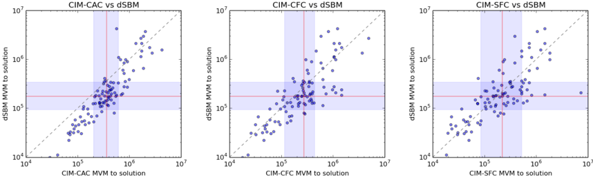
The image presents three scatter plots comparing the performance of different CIM (Combinatorial Interaction Modeling) methods against a dSBM (degree-corrected stochastic block model) approach. Each plot compares a specific CIM variant (CAC, CFC, SFC) against dSBM in terms of "MVM to solution," likely referring to a measure of computational effort or resources required to reach a solution. The plots use a log-log scale, and each includes a dashed diagonal line, a horizontal line, and a vertical line, along with shaded regions.
### Components/Axes
* **Titles:**
* Left Plot: "CIM-CAC vs dSBM"
* Middle Plot: "CIM-CFC vs dSBM"
* Right Plot: "CIM-SFC vs dSBM"
* **X-axis (all plots):**
* Label: "CIM-[Variant] MVM to solution" (where [Variant] is CAC, CFC, or SFC)
* Scale: Logarithmic, ranging from 10^4 to 10^7
* Ticks: 10^4, 10^5, 10^6, 10^7
* **Y-axis (all plots):**
* Label: "dSBM MVM to solution"
* Scale: Logarithmic, ranging from 10^4 to 10^7
* Ticks: 10^4, 10^5, 10^6, 10^7
* **Data Points:** Blue dots representing individual data points.
* **Diagonal Line:** Dashed gray line representing the line of equality (x=y).
* **Horizontal Line:** Solid red line, indicating a specific dSBM MVM value. Appears to be around 2 * 10^5.
* **Vertical Line:** Solid red line, indicating a specific CIM MVM value. Appears to be around 2 * 10^5.
* **Shaded Regions:** Light blue shaded regions around the horizontal and vertical lines, indicating a range or tolerance around those values.
### Detailed Analysis
**Plot 1: CIM-CAC vs dSBM**
* **X-axis:** CIM-CAC MVM to solution
* **Y-axis:** dSBM MVM to solution
* **Data Points:** The blue data points are clustered around the intersection of the red lines, with a spread both above and below the diagonal line.
* **Trend:** The data points generally follow a positive correlation, but with significant scatter.
* **Horizontal Line:** Located at approximately 2 * 10^5 on the Y-axis.
* **Vertical Line:** Located at approximately 2 * 10^5 on the X-axis.
**Plot 2: CIM-CFC vs dSBM**
* **X-axis:** CIM-CFC MVM to solution
* **Y-axis:** dSBM MVM to solution
* **Data Points:** Similar to the first plot, the data points are clustered around the intersection of the red lines, with a spread both above and below the diagonal line.
* **Trend:** The data points generally follow a positive correlation, but with significant scatter.
* **Horizontal Line:** Located at approximately 2 * 10^5 on the Y-axis.
* **Vertical Line:** Located at approximately 2 * 10^5 on the X-axis.
**Plot 3: CIM-SFC vs dSBM**
* **X-axis:** CIM-SFC MVM to solution
* **Y-axis:** dSBM MVM to solution
* **Data Points:** Similar to the first two plots, the data points are clustered around the intersection of the red lines, with a spread both above and below the diagonal line.
* **Trend:** The data points generally follow a positive correlation, but with significant scatter.
* **Horizontal Line:** Located at approximately 2 * 10^5 on the Y-axis.
* **Vertical Line:** Located at approximately 2 * 10^5 on the X-axis.
### Key Observations
* All three plots show a similar pattern: a cluster of data points around the intersection of the red lines, with a general positive correlation between the CIM variant and dSBM.
* The scatter around the diagonal line suggests that the performance of the CIM variants and dSBM can vary significantly for individual instances.
* The red lines and shaded regions appear to highlight a specific performance range or target.
### Interpretation
The plots compare the "MVM to solution" (likely a measure of computational effort) for different CIM methods (CAC, CFC, SFC) against dSBM. The clustering of data points around the intersection of the red lines suggests that, on average, the CIM variants and dSBM have similar performance characteristics within the range defined by the red lines and shaded regions. However, the significant scatter indicates that the relative performance of these methods can vary considerably depending on the specific problem instance. The diagonal line represents the ideal scenario where both methods have equal "MVM to solution." Points above the line indicate that dSBM requires more effort, while points below the line indicate that the CIM variant requires more effort. The shaded regions likely represent a tolerance or acceptable range of performance.