## Scatter Plot Comparison: CIM Variants vs dSBM
### Overview
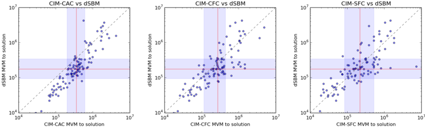
The image displays three side-by-side scatter plots comparing the performance (measured in "MVM to solution") of three different CIM (likely a computational method) variants against a baseline dSBM method. Each plot uses a log-log scale. The data points represent individual problem instances or runs. Reference lines and shaded regions indicate central tendency and spread.
### Components/Axes
* **Titles (Top-Center of each plot):**
* Left Plot: `CIM-CAC vs dSBM`
* Middle Plot: `CIM-CFC vs dSBM`
* Right Plot: `CIM-SFC vs dSBM`
* **X-Axis Label (Bottom of each plot):** `CIM-[VARIANT] MVM to solution`
* Left: `CIM-CAC MVM to solution`
* Middle: `CIM-CFC MVM to solution`
* Right: `CIM-SFC MVM to solution`
* **Y-Axis Label (Left of each plot):** `dSBM MVM to solution`
* **Axis Scales:** Logarithmic, ranging from `10^4` to `10^7` on both axes for all plots.
* **Data Series:** Blue circular dots, one per data point.
* **Reference Elements:**
* **Diagonal Dashed Line:** A `y = x` line indicating equal performance between the two methods.
* **Red Solid Lines:** A vertical and a horizontal line intersecting, likely marking the median or mean of each distribution.
* **Light Blue Shaded Regions:** A vertical and a horizontal band, likely representing the interquartile range (IQR) or a similar measure of spread for each method's distribution.
### Detailed Analysis
**1. Left Plot: CIM-CAC vs dSBM**
* **Trend:** Data points cluster tightly along the `y = x` diagonal line, indicating strong agreement in performance between CIM-CAC and dSBM for most instances.
* **Central Tendency (Red Lines):** The intersection is approximately at `(2.0 x 10^5, 2.0 x 10^5)`.
* **Spread (Shaded Regions):**
* Vertical band (CIM-CAC spread): Spans roughly from `1.5 x 10^5` to `3.0 x 10^5`.
* Horizontal band (dSBM spread): Spans roughly from `1.5 x 10^5` to `3.0 x 10^5`.
* **Outliers:** A few points lie noticeably above the diagonal in the upper-right quadrant (e.g., near `(2.0 x 10^6, 4.0 x 10^6)`), suggesting dSBM was slower for those specific cases.
**2. Middle Plot: CIM-CFC vs dSBM**
* **Trend:** Data points show a positive correlation but with significantly more scatter away from the `y = x` line compared to the left plot. Many points lie above the diagonal.
* **Central Tendency (Red Lines):** The intersection is approximately at `(1.8 x 10^5, 2.0 x 10^5)`.
* **Spread (Shaded Regions):**
* Vertical band (CIM-CFC spread): Spans roughly from `1.0 x 10^5` to `3.5 x 10^5`. This band is wider than in the left plot.
* Horizontal band (dSBM spread): Spans roughly from `1.5 x 10^5` to `3.0 x 10^5`.
* **Outliers:** Several points are far above the diagonal, particularly in the range where CIM-CFC is `10^5` to `10^6`, indicating instances where dSBM required 2-10 times more MVMs. One point is near `(1.0 x 10^6, 8.0 x 10^6)`.
**3. Right Plot: CIM-SFC vs dSBM**
* **Trend:** Data points show a positive correlation with scatter intermediate between the left and middle plots. A subset of points lies above the diagonal.
* **Central Tendency (Red Lines):** The intersection is approximately at `(1.8 x 10^5, 2.0 x 10^5)`.
* **Spread (Shaded Regions):**
* Vertical band (CIM-SFC spread): Spans roughly from `1.2 x 10^5` to `3.0 x 10^5`.
* Horizontal band (dSBM spread): Spans roughly from `1.5 x 10^5` to `3.0 x 10^5`.
* **Outliers:** A few points are significantly above the diagonal, with one notable point near `(1.5 x 10^6, 2.0 x 10^6)`.
### Key Observations
1. **Performance Hierarchy:** The tightness of clustering around the diagonal suggests the following order in terms of performance similarity to dSBM: **CIM-CAC (most similar) > CIM-SFC > CIM-CFC (least similar)**.
2. **Systematic Bias:** In the CIM-CFC and CIM-SFC plots, a noticeable number of points lie *above* the diagonal. This indicates a trend where, for those instances, the dSBM method required more MVMs (was slower) than the CIM variant.
3. **Consistent dSBM Spread:** The horizontal red line and shaded band for dSBM are in nearly identical positions across all three plots, confirming it is the consistent baseline.
4. **Varying CIM Spread:** The vertical spread (performance variability) of the CIM methods differs: CIM-CFC shows the widest spread, followed by CIM-SFC, with CIM-CAC being the most consistent.
### Interpretation
This analysis compares the computational effort (MVMs to solution) of three algorithmic variants (CIM-CAC, CIM-CFC, CIM-SFC) against a standard (dSBM). The data suggests:
* **CIM-CAC is a robust alternative to dSBM,** yielding nearly identical performance on most problem instances. It is a reliable drop-in replacement.
* **CIM-CFC and CIM-SFC offer potential performance gains** but with trade-offs. They frequently solve instances with fewer MVMs than dSBM (points above the diagonal), but their performance is more variable (wider vertical spread). CIM-CFC shows the highest potential for speedup but also the highest variability and risk of underperformance.
* The **outliers above the diagonal are significant**. They represent specific problem structures where the CIM approach (especially CFC and SFC) is substantially more efficient than the dSBM approach. Investigating these instances could reveal the strengths of the CIM methodology.
* The **log-log scale** is crucial, as it shows that performance differences are often multiplicative (factors of 2x, 5x, 10x) rather than additive.
In essence, the charts demonstrate that while CIM-CAC matches dSBM's reliability, the CIM-CFC and CIM-SFC variants introduce a performance-variance trade-off, offering the possibility of significant speedups on a subset of problems at the cost of less predictable performance overall.