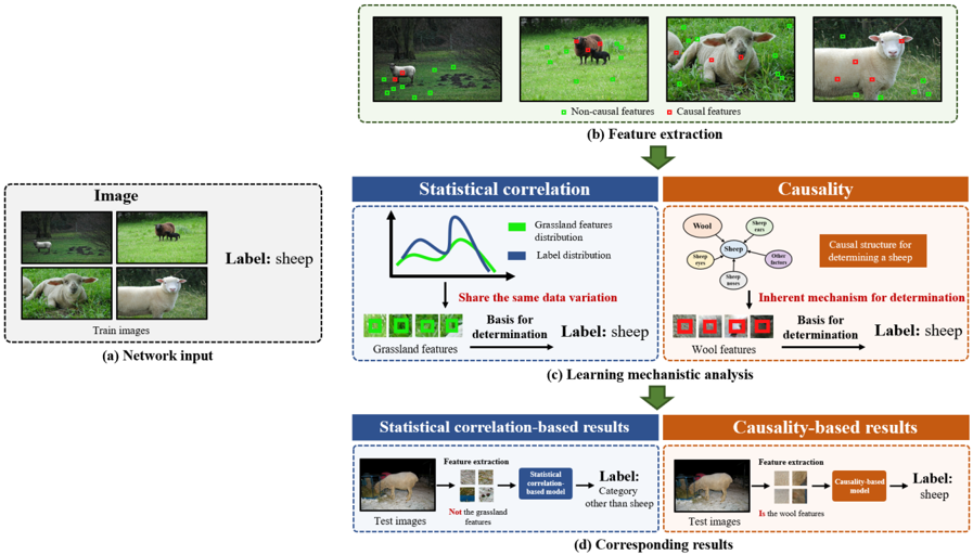
## Diagram: Learning Mechanism Analysis for Sheep Classification (Statistical Correlation vs. Causality) ### Overview This image is a conceptual diagram illustrating and contrasting two approaches to machine learning for image classification, using "sheep" as the example class. It demonstrates how a model relying on **statistical correlation** (e.g., associating sheep with grassland) can fail, while a model based on **causality** (identifying inherent sheep features like wool) is more robust. The diagram flows from input data, through feature extraction and learning analysis, to final classification results. ### Components/Axes The diagram is organized into four main labeled sections, flowing top to bottom: 1. **(a) Network input**: A dashed box containing four "Train images" of sheep in various outdoor settings (grassland, field). The overarching label is "Label: sheep". 2. **(b) Feature extraction**: A dashed box showing the same four images overlaid with colored squares. A legend defines: * **Green squares**: "Non-causal features" * **Red squares**: "Causal features" * The red squares are consistently placed on the sheep's body/face, while green squares are on the background grass/ground. 3. **(c) Learning mechanistic analysis**: The core analytical section, split into two parallel columns: * **Left Column (Blue Header)**: "Statistical correlation" * Contains a line graph with two curves: a green line labeled "Grassland features distribution" and a blue line labeled "Label distribution". The x-axis is unlabeled but implies feature space; the y-axis is unlabeled but implies frequency/probability. The curves show a strong overlap. * Below the graph: Text "Share the same data variation". * Below that: A row of green squares labeled "Grassland features" pointing via an arrow labeled "Basis for determination" to the text "Label: sheep". * **Right Column (Orange Header)**: "Causality" * Contains a causal diagram (graph) with a central node "sheep" connected to nodes: "Wool", "Sheep face", "Sheep ears", "Sheep nose", "Sheep legs". * A text box states: "Causal structure for determining a sheep". * Below the diagram: Text "Inherent mechanism for determination". * Below that: A row of red squares (showing sheep features) labeled "Wool features" pointing via an arrow labeled "Basis for determination" to the text "Label: sheep". 4. **(d) Corresponding results**: Shows the outcome of each approach on a "Test image" (a sheep on a dirt path, not grass). * **Left (Statistical correlation-based results)**: The test image goes through "Feature extraction" yielding green squares (grassland features). The text notes "Not the grassland features". This feeds into a "Statistical correlation-based model", which outputs "Label: Category other than sheep". * **Right (Causality-based results)**: The same test image goes through "Feature extraction" yielding red squares (wool features). The text notes "Is the wool features". This feeds into a "Causality-based model", which outputs "Label: sheep". ### Detailed Analysis * **Feature Extraction (b)**: The diagram explicitly defines which visual elements are considered causal (red, on the animal) versus non-causal (green, on the background). This is a critical interpretive key for the rest of the diagram. * **Learning Mechanism (c)**: * The **Statistical Correlation** model learns that the presence of "Grassland features" (green) co-varies perfectly with the "Label: sheep" in the training data. The graph visually represents this as two distributions that "share the same data variation." Its basis for determination is the background context. * The **Causality** model learns an "Inherent mechanism" represented by a causal graph. It identifies core attributes of the object itself ("Wool", "Sheep face", etc.) as the basis for determination, independent of background. * **Results (d)**: This section provides the logical conclusion. The test image lacks the strong grassland background present in training. * The **Statistical correlation-based model** fails because its learned basis ("grassland features") is absent. It extracts the wrong features (green squares) and misclassifies. * The **Causality-based model** succeeds because its learned basis ("wool features") is present on the test sheep. It extracts the correct features (red squares) and classifies correctly. ### Key Observations 1. **Spatial Grounding of Features**: The red "causal" squares are consistently located on the sheep's body across all images in (b) and (d), while green "non-causal" squares are on the environment. 2. **Trend Verification**: The line graph in the statistical correlation column shows both distributions peaking and dipping together, visually confirming the "share the same data variation" claim. 3. **Component Isolation**: The diagram cleanly isolates the input, feature extraction, learning theory, and practical results into distinct, connected blocks. 4. **Color Consistency**: The color coding (green=non-causal/grassland, red=causal/wool) is maintained strictly throughout all sections (b), (c), and (d), allowing for clear cross-referencing. ### Interpretation This diagram is an **argument for causal representation learning in computer vision**. It posits that models which learn superficial statistical correlations (sheep are often on grass) are brittle and fail when test data deviates from the training distribution (a sheep not on grass). In contrast, models that learn the **inherent causal structure** of an object (sheep have wool, specific facial features) are more robust and generalize better. The "Peircean" investigative reading here is that the diagram uses a **hypothetico-deductive structure**: * **Hypothesis**: Causality-based learning is superior to correlation-based learning. * **Experiment Setup**: Shown in (a) and (b) - training data with confounding background features. * **Theoretical Framework**: Shown in (c) - the two competing learning mechanisms. * **Deductive Prediction & Test**: Shown in (d) - applying both models to a challenging test case. * **Conclusion**: The result validates the hypothesis, as only the causality-based model performs correctly. The underlying message is about **disentanglement**: separating the true object features (causal) from spurious environmental correlations (non-causal) is key to building reliable and generalizable AI systems. The diagram serves as a clear, visual pedagogical tool to explain this complex concept.