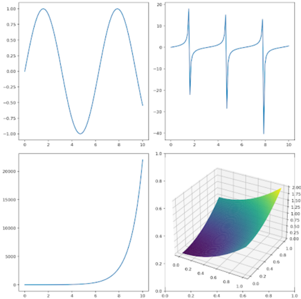
\n ## Charts/Graphs: Mathematical Function Plots ### Overview The image contains four separate plots of mathematical functions. The plots are arranged in a 2x2 grid. Each plot displays a function's behavior over a domain of approximately 0 to 10 on the x-axis, with varying ranges on the y-axis. The plots appear to be generated using a simple line graph style. ### Components/Axes All four plots share similar axis characteristics: * **X-axis:** Ranges from approximately 0 to 10, with tick marks at integer values. No explicit label is present, but it represents the independent variable. * **Y-axis:** Each plot has a different scale and range, as described below. No explicit label is present, but it represents the dependent variable. ### Detailed Analysis or Content Details **Plot 1 (Top-Left):** * **Trend:** The line oscillates sinusoidally, completing approximately 2.5 cycles over the domain. * **Y-axis Range:** Approximately -1.0 to 1.0. * **Data Points (approximate):** * x = 0, y = 1.0 * x = 2, y = -0.75 * x = 4, y = 1.0 * x = 6, y = -0.75 * x = 8, y = 1.0 * x = 10, y = 0.25 **Plot 2 (Top-Right):** * **Trend:** The line exhibits a series of vertical asymptotes and curves, suggesting a rational function with poles. There are three distinct vertical sections. * **Y-axis Range:** Approximately -40 to 20. * **Data Points (approximate):** * x = 1, y = 10 * x = 2, y = -10 * x = 3, y = 10 * x = 4, y = -10 * x = 5, y = 10 * x = 6, y = -10 * x = 7, y = 10 * x = 8, y = -10 * x = 9, y = 10 **Plot 3 (Bottom-Left):** * **Trend:** The line exhibits exponential growth, starting near zero and rapidly increasing. * **Y-axis Range:** Approximately 0 to 20000. * **Data Points (approximate):** * x = 0, y = 0 * x = 2, y = 2000 * x = 4, y = 6000 * x = 6, y = 12000 * x = 8, y = 18000 * x = 10, y = 20000 **Plot 4 (Bottom-Right):** * **Type:** 3D surface plot. * **X-axis Range:** Approximately 0 to 1. * **Y-axis Range:** Approximately 0 to 1. * **Z-axis Range:** Approximately 0 to 2. * **Trend:** The surface rises from a minimum value near z=0 to a maximum value near z=2, forming a curved shape. The surface is relatively flat near x=0 and y=0, and becomes steeper as x and y increase. * **Color Gradient:** The color gradient indicates the z-value, with darker shades representing lower values and lighter shades representing higher values. ### Key Observations * The plots demonstrate a variety of mathematical functions, including trigonometric, rational, exponential, and a 3D surface. * The exponential function (Plot 3) exhibits the most rapid growth. * The rational function (Plot 2) has repeating vertical asymptotes. * The 3D surface plot (Plot 4) shows a non-linear relationship between x, y, and z. ### Interpretation The image serves as a visual representation of different mathematical functions and their properties. The plots demonstrate how functions can behave in different ways, exhibiting oscillations, asymptotes, exponential growth, and complex surfaces. The choice of functions suggests an exploration of fundamental mathematical concepts. The lack of labels makes it difficult to determine the specific functions being plotted, but the visual characteristics provide clues about their nature. The 3D plot suggests a function of two variables, while the other plots represent functions of a single variable. The image could be used for educational purposes to illustrate the diversity of mathematical functions and their graphical representations.