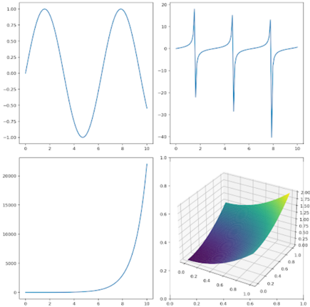
## Mathematical Function Plots: 2x2 Grid Analysis ### Overview The image displays a 2x2 grid of four distinct mathematical function plots, each rendered in a standard scientific plotting style with blue lines on a white background. The plots appear to be generated by a library like Matplotlib. There are no overall titles, axis labels, or legends present, requiring inference from the visual data. ### Components/Axes The image is segmented into four quadrants: 1. **Top-Left:** A 2D line plot of a periodic function. 2. **Top-Right:** A 2D line plot of a function with sharp discontinuities or high-frequency oscillations. 3. **Bottom-Left:** A 2D line plot of a rapidly growing function. 4. **Bottom-Right:** A 3D surface plot. **Common Axes Characteristics:** * All 2D plots share an x-axis range of approximately **0 to 10**. * The y-axis scales differ significantly between plots. * Axis tick marks are present, but axis titles and plot titles are absent. ### Detailed Analysis #### 1. Top-Left Plot: Periodic Waveform * **Visual Trend:** A smooth, symmetric, periodic wave resembling a sine or cosine function. * **Axes:** * X-axis: Linear scale, ticks at 0, 2, 4, 6, 8, 10. * Y-axis: Linear scale, ticks at -1.00, -0.75, -0.50, -0.25, 0.00, 0.25, 0.50, 0.75, 1.00. * **Data Points & Key Features:** * **Amplitude:** Approximately **1.0** (peak at ~1.0, trough at ~-1.0). * **Period:** Approximately **6.3 units** (peak-to-peak distance from x≈2 to x≈8.3). * **Phase:** Starts near y=0 at x=0, rising to a first peak at **x ≈ 2.0, y ≈ 1.0**. * Crosses zero at **x ≈ 3.6** and **x ≈ 6.8**. * Minimum (trough) at **x ≈ 5.2, y ≈ -1.0**. #### 2. Top-Right Plot: Discontinuous/Oscillatory Function * **Visual Trend:** A function characterized by sharp, narrow downward spikes (troughs) and broader upward peaks, suggesting a derivative of a discontinuous function or a function like `tan(x)` or `1/sin(x)`. * **Axes:** * X-axis: Linear scale, ticks at 0, 2, 4, 6, 8, 10. * Y-axis: Linear scale, ticks at -40, -30, -20, -10, 0, 10, 20. * **Data Points & Key Features:** * **Three prominent downward spikes** (local minima) are visible: 1. **x ≈ 1.5, y ≈ -38** (approximate, deepest spike). 2. **x ≈ 4.7, y ≈ -28**. 3. **x ≈ 7.9, y ≈ -18**. * **Three corresponding upward peaks** (local maxima) precede each spike: 1. **x ≈ 1.2, y ≈ 18**. 2. **x ≈ 4.4, y ≈ 15**. 3. **x ≈ 7.6, y ≈ 12**. * The function appears to approach **y=0** asymptotically between these features. #### 3. Bottom-Left Plot: Exponential Growth * **Visual Trend:** A curve showing very slow initial growth followed by extremely rapid, accelerating increase, characteristic of an exponential or high-order polynomial function. * **Axes:** * X-axis: Linear scale, ticks at 0, 2, 4, 6, 8, 10. * Y-axis: Linear scale, ticks at 0, 5000, 10000, 15000, 20000. * **Data Points & Key Features:** * For **x < 6**, the y-value remains very low, visually close to **0**. * The curve begins a noticeable rise around **x ≈ 6**. * Growth becomes explosive after **x ≈ 8**. * At the right edge (**x = 10**), the y-value is approximately **20,000** (the top of the axis range). #### 4. Bottom-Right Plot: 3D Surface * **Visual Trend:** A smooth, curved surface in 3D space, showing a monotonic increase in the z-value as both x and y increase. The color gradient (blue to yellow) reinforces the height (z-value). * **Axes & Components:** * **X-axis (left-bottom):** Linear scale from **0.0 to 1.0**, ticks at 0.0, 0.2, 0.4, 0.6, 0.8, 1.0. * **Y-axis (right-bottom):** Linear scale from **0.0 to 1.0**, ticks at 0.0, 0.2, 0.4, 0.6, 0.8, 1.0. * **Z-axis (vertical):** Linear scale from **0.0 to 2.0**, ticks at 0.0, 0.25, 0.50, 0.75, 1.00, 1.25, 1.50, 1.75, 2.00. * **Color Mapping:** The surface uses a colormap (likely 'viridis' or similar). **Dark blue/purple** corresponds to low z-values (~0.0-0.5), transitioning through **teal/green** to **bright yellow** for high z-values (~1.5-2.0). * **Surface Shape & Key Points:** * The surface is lowest (dark blue) at the corner **(x=0.0, y=0.0)**, where **z ≈ 0.0**. * It rises smoothly and convexly. * The highest point (bright yellow) is at the opposite corner **(x=1.0, y=1.0)**, where **z ≈ 2.0**. * The surface appears to be defined by a function like **z = x + y** or **z = 2*max(x,y)**, given the linear-looking rise along the diagonal. ### Key Observations 1. **Scale Disparity:** The y-axis scales vary by orders of magnitude across the 2D plots (from ~±1 to ~20,000), indicating vastly different function behaviors. 2. **Functional Diversity:** The four plots showcase fundamentally different mathematical behaviors: periodic, discontinuous/singular, explosive growth, and multi-variable dependence. 3. **Missing Metadata:** The complete lack of titles, axis labels, and legends is a significant omission for a technical document, forcing all interpretation to be based solely on the visual form of the data. 4. **3D Visualization:** The bottom-right plot effectively uses both spatial perspective and color to encode a third dimension (z-value). ### Interpretation This grid likely serves as a **comparative visualization of different function classes** or **test cases for a plotting system**. It demonstrates the system's ability to handle: * Standard 2D plotting with varying data ranges. * Functions with sharp features or potential singularities. * Data requiring large y-axis scales. * 3D surface rendering with color mapping. The absence of labels suggests this might be a preliminary output, a figure from a context where the functions are defined elsewhere (e.g., a code notebook), or a test image for evaluating rendering capabilities. The stark contrast between the smooth periodic wave and the spiky discontinuous function highlights the importance of choosing appropriate visualization methods for different data types. The exponential plot warns of the visual challenges in plotting data with extreme dynamic ranges on a linear scale. The 3D plot provides an intuitive understanding of a bivariate relationship that would be difficult to convey with 2D plots alone. Collectively, they represent a foundational toolkit for visualizing mathematical and scientific data.