## Line Chart: Completeness vs. Samples for Two Parameter Sets
### Overview
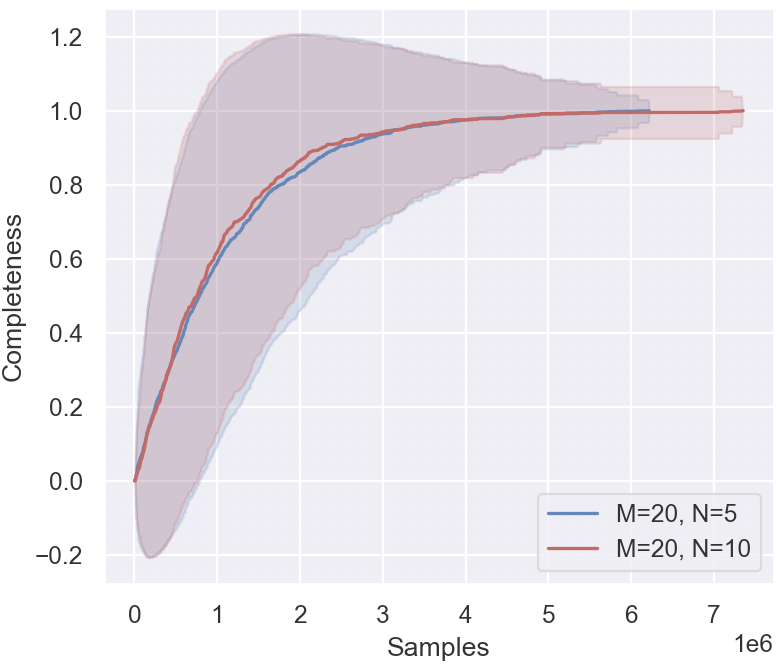
The image displays a line chart plotting "Completeness" against the number of "Samples" for two different experimental conditions. Each condition is represented by a central trend line and a shaded region indicating the confidence interval or variance around that trend. The chart demonstrates how a completeness metric evolves and converges as the number of samples increases.
### Components/Axes
* **Chart Type:** Line chart with shaded confidence intervals.
* **X-Axis:**
* **Label:** "Samples"
* **Scale:** Linear scale from 0 to 7,000,000 (7 x 10⁶). Major tick marks are at 0, 1, 2, 3, 4, 5, 6, and 7 million.
* **Y-Axis:**
* **Label:** "Completeness"
* **Scale:** Linear scale from -0.2 to 1.2. Major tick marks are at -0.2, 0.0, 0.2, 0.4, 0.6, 0.8, 1.0, and 1.2.
* **Legend:**
* **Position:** Bottom-right corner of the plot area.
* **Entries:**
1. **Blue Line:** Label "M=20, N=5"
2. **Red Line:** Label "M=20, N=10"
* **Data Series:**
1. **Series 1 (Blue):** Corresponds to "M=20, N=5". Consists of a solid blue central line and a light blue shaded confidence band.
2. **Series 2 (Red):** Corresponds to "M=20, N=10". Consists of a solid red central line and a light red/pink shaded confidence band.
### Detailed Analysis
**Trend Verification & Data Points:**
* **Both Series Trend:** Both the blue and red lines exhibit a logarithmic-like growth pattern. They start near a completeness of 0.0 at 0 samples, rise steeply initially, and then gradually plateau, approaching an asymptote near a completeness value of 1.0.
* **Blue Line (M=20, N=5):**
* **Trend:** Slopes upward sharply from the origin, crossing 0.4 completeness at ~500,000 samples, 0.8 at ~2,000,000 samples, and 0.95 at ~4,000,000 samples. It appears to plateau very close to 1.0 from approximately 5,000,000 samples onward.
* **Confidence Interval (Blue Shading):** The shaded region is very wide at low sample counts, spanning from approximately -0.2 to +1.2 at its peak around 1,000,000 samples. This indicates high variance or uncertainty in the early stages. The band narrows significantly as samples increase, becoming a tight band around the central line after ~4,000,000 samples.
* **Red Line (M=20, N=10):**
* **Trend:** Follows a very similar path to the blue line but appears to rise slightly faster in the initial phase (0 to 1,500,000 samples). It crosses 0.4 completeness at ~400,000 samples and 0.8 at ~1,800,000 samples. It converges with the blue line's trajectory around 3,000,000 samples and plateaus at the same level (~1.0).
* **Confidence Interval (Red Shading):** The shaded region is also wide initially but appears slightly narrower than the blue band in the very early stage (0-500,000 samples). It narrows as samples increase, following a similar convergence pattern to the blue band.
### Key Observations
1. **Convergence:** Both parameter sets (M=20 with N=5 and N=10) lead to the same final completeness level (~1.0) given a sufficient number of samples (approximately 5 million or more).
2. **Early-Stage Difference:** The series with N=10 (red) shows a marginally faster initial increase in completeness compared to N=5 (blue) for the same number of samples below ~2 million.
3. **High Initial Variance:** Both series exhibit extremely high variance (wide confidence intervals) when the sample count is low (< 2 million), suggesting the completeness metric is highly unstable or uncertain with sparse data.
4. **Stability with Scale:** The variance diminishes dramatically as the sample size grows, indicating the measurement becomes stable and reliable with large datasets.
5. **Parameter Impact:** Holding M constant at 20, increasing N from 5 to 10 appears to improve the *rate* of completeness acquisition in the data-scarce regime but does not affect the ultimate achievable completeness.
### Interpretation
This chart likely illustrates the performance of a sampling-based algorithm or estimation process where "Completeness" measures how much of the target information or solution space has been captured. The parameters M and N could represent dimensions of the problem, such as the number of features (M) and the number of samples per feature or a similar constraint (N).
The data suggests that **increasing the sample size is the primary driver for achieving high completeness**, with both configurations eventually reaching near-perfect completeness (~1.0). The **parameter N influences efficiency**: a higher N (10 vs. 5) provides a slight advantage in the early learning phase, allowing the system to reach a given completeness level with fewer samples. However, this advantage diminishes as the sample count grows large.
The **massive initial confidence intervals** are a critical finding. They imply that any single run or small set of runs with fewer than ~2 million samples could yield wildly different completeness scores, from near-zero to near-perfect. This highlights the necessity of large sample sizes not just for high completeness, but for *reliable and reproducible* results. The convergence of both the means and the confidence bands at high sample counts indicates the process becomes deterministic and predictable with enough data.
**In summary:** For this system, prioritize collecting a large number of samples (>5 million) to guarantee high and stable completeness. If computational resources are limited and only a smaller sample budget is available (<2 million), using the configuration with the higher N value (N=10) may yield slightly better, though still highly variable, results.