TECHNICAL ASSET FINGERPRINT
c3386db7b0abc4f41e5f392e
Click to view fullscreen
Press ESC or click to close
FOUND IN PAPERS
EXPERT: healer-alpha-free VERSION 1
RUNTIME: free/openrouter/healer-alpha
INTEL_VERIFIED
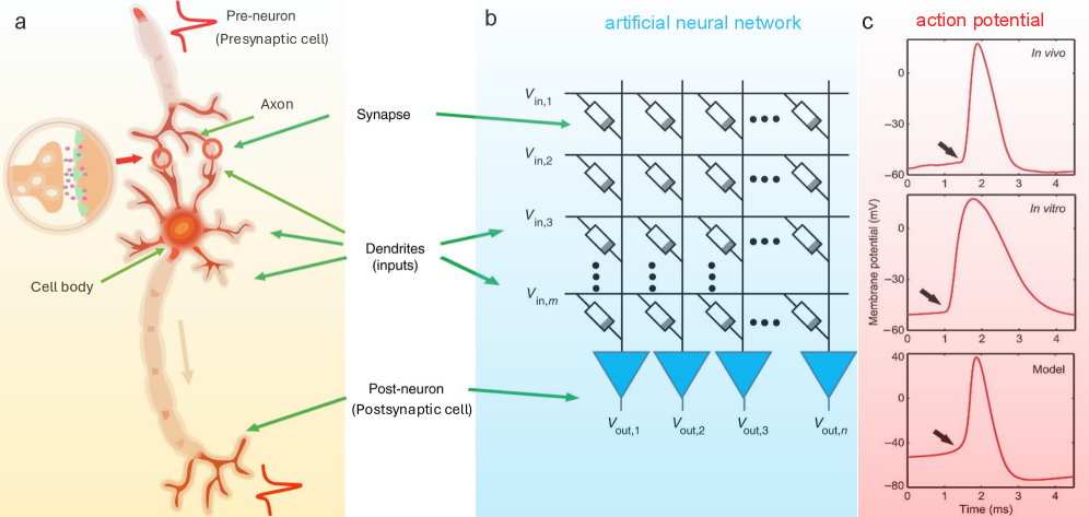
## [Scientific Diagram]: Comparison of Biological Neuron, Artificial Neural Network, and Action Potential Waveforms
### Overview
The image is a three-panel scientific figure (labeled a, b, c) illustrating the analogy between a biological neuron, an artificial neural network (ANN) architecture, and the resulting action potential waveforms. Panel (a) depicts a biological neuron with its key components. Panel (b) shows a schematic of an artificial neural network layer, mapping biological components to artificial ones. Panel (c) presents three graphs comparing action potential waveforms from different sources: *in vivo*, *in vitro*, and a computational model.
### Components/Axes
**Panel (a): Biological Neuron**
* **Main Labels (with approximate positions):**
* `Pre-neuron (Presynaptic cell)`: Top-left, pointing to the axon terminal of a preceding neuron.
* `Axon`: Upper-middle, pointing to the long projection from the cell body.
* `Synapse`: Middle, pointing to the junction between the axon terminal and the dendrite.
* `Dendrites (inputs)`: Middle-right, pointing to the branching input structures of the neuron.
* `Cell body`: Center-left, pointing to the main soma of the neuron.
* `Post-neuron (Postsynaptic cell)`: Bottom-right, pointing to the axon terminal of the depicted neuron, indicating it connects to a subsequent cell.
* **Inset:** A circular inset on the left shows a magnified view of a synapse, with a red arrow pointing from it to the synapse label on the main neuron diagram.
**Panel (b): Artificial Neural Network**
* **Title:** `artificial neural network` (top center, in blue).
* **Input Labels (Left side, vertical column):**
* `V_in,1`
* `V_in,2`
* `V_in,3`
* `V_in,m` (indicating an arbitrary number of inputs).
* **Output Labels (Bottom, horizontal row):**
* `V_out,1`
* `V_out,2`
* `V_out,3`
* `V_out,n` (indicating an arbitrary number of outputs).
* **Structure:** A grid of horizontal and vertical lines. At each intersection is a rectangular symbol representing a resistor or synaptic weight. The vertical lines terminate in downward-pointing blue triangles, representing output neurons or activation functions.
* **Mapping Arrows:** Green arrows connect labels from panel (a) to panel (b):
* `Synapse` → points to a resistor symbol in the grid.
* `Dendrites (inputs)` → points to the `V_in` labels.
* `Post-neuron (Postsynaptic cell)` → points to the blue triangle output units.
**Panel (c): Action Potential Graphs**
* **Title:** `action potential` (top center, in red).
* **Three vertically stacked graphs.** Each shares the same axes:
* **Y-axis:** `Membrane potential (mV)`. Scale ranges from approximately -80 mV to +40 mV.
* **X-axis:** `Time (ms)`. Scale ranges from 0 to 4 ms.
* **Graph Labels (Top-right of each plot):**
* Top graph: `In vivo`
* Middle graph: `In vitro`
* Bottom graph: `Model`
* **Data Series:** Each graph contains a single red line plotting membrane potential over time. A black arrow in each graph points to the initial depolarization phase (the "foot" of the action potential).
### Detailed Analysis
**Panel (a) - Biological Neuron:**
The diagram shows a typical multipolar neuron. The signal flow is implied: input arrives at the dendrites/cell body from a pre-neuron via a synapse, is processed, and an output signal travels down the axon to the next (post-) neuron. The inset clarifies the synaptic cleft structure.
**Panel (b) - Artificial Neural Network:**
This is a schematic of a fully connected layer or a crossbar array, often used in neuromorphic engineering. Each `V_in` is connected to each output unit via a programmable weight (the resistor symbol). The output `V_out,j` is likely a function of the weighted sum of inputs. The green arrows explicitly map the biological concepts (synapse = weight, dendrites = input lines, post-neuron = output unit) to the artificial construct.
**Panel (c) - Action Potential Waveforms:**
* **Trend Verification:** All three waveforms show the classic action potential shape: a rapid depolarization (rising phase) to a peak, followed by repolarization (falling phase) and a hyperpolarization undershoot before returning to resting potential (~-60 to -70 mV).
* **Data Point Extraction (Approximate):**
* **Resting Potential:** ~ -65 mV for all three.
* **Peak Depolarization:**
* `In vivo`: ~ +35 mV
* `In vitro`: ~ +30 mV
* `Model`: ~ +40 mV
* **Timing:** The action potential begins at ~1 ms and peaks at ~1.5-2 ms in all cases. The duration (width at half-maximum) appears slightly broader in the `In vitro` trace compared to the `In vivo` and `Model` traces.
* **Key Feature (Arrows):** The black arrows highlight the pre-potential or "foot" of the action potential, a small depolarization before the rapid upstroke, which is present in all three traces.
### Key Observations
1. **Direct Analogy:** The figure constructs a clear visual analogy: Biological Neuron (a) → Artificial Network Model (b) → Functional Output (c).
2. **Waveform Similarity:** The action potential waveforms from the biological sources (*in vivo*, *in vitro*) and the computational `Model` are qualitatively very similar, suggesting the model successfully captures the essential dynamics.
3. **Minor Discrepancies:** The `Model` produces a slightly higher peak depolarization (+40 mV) compared to the biological examples (+30 to +35 mV). The `In vitro` waveform shows a slightly more pronounced after-hyperpolarization (dip below resting potential).
4. **Spatial Grounding:** The legend/labels are consistently placed: titles at the top of each panel, axis labels on the left and bottom of graphs, and component labels adjacent to their targets with guiding arrows.
### Interpretation
This figure serves as a pedagogical or conceptual bridge between neuroscience and artificial intelligence/neuromorphic engineering. It demonstrates how the fundamental information-processing unit of the brain (the neuron) is abstracted into a mathematical/computational model (the ANN layer). The action potential graphs in panel (c) validate the model by showing it can reproduce the key electrophysiological signature of a biological neuron.
The **Peircean investigative reading** reveals:
* **Iconic Sign:** The diagrams in (a) and (b) are icons—they resemble their real-world counterparts (a neuron, a circuit).
* **Indexical Sign:** The green arrows are indices—they point directly from the biological feature to its artificial analogue, establishing a causal or correlational relationship.
* **Symbolic Sign:** The labels (`V_in`, `mV`, `ms`) and the graph itself are symbols, relying on shared scientific convention to convey precise meaning.
The underlying message is one of biomimicry: by understanding and replicating the structure (panels a & b) of biological neural systems, we can recreate their functional dynamics (panel c). The minor discrepancies between the `Model` and biological traces highlight areas for potential model refinement, such as adjusting parameters to match peak amplitude or repolarization kinetics more precisely. The figure argues for the validity of the artificial construct by grounding it in observable biological data.
DECODING INTELLIGENCE...