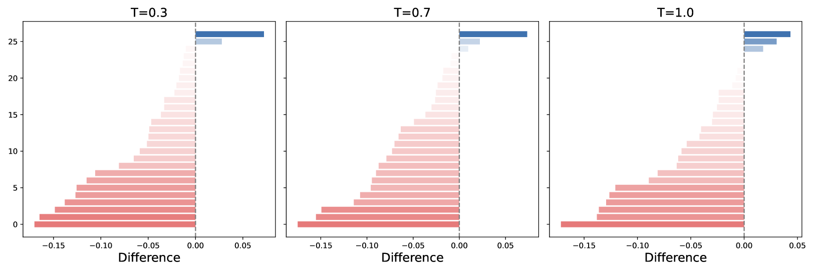
\n ## Histograms: Distribution of Differences at Varying Time Points ### Overview The image presents three histograms, each representing the distribution of "Difference" values at different time points (T = 0.3, T = 0.7, and T = 1.0). The histograms are visually similar, displaying a right-skewed distribution with a concentration of values near zero and a tail extending towards positive differences. The y-axis represents a count or frequency, while the x-axis represents the "Difference" value. ### Components/Axes * **X-axis Label:** "Difference" * **Y-axis:** Count/Frequency (unlabeled, but implied) * **Titles:** * Left Histogram: "T=0.3" * Center Histogram: "T=0.7" * Right Histogram: "T=1.0" * **X-axis Range:** Approximately -0.15 to 0.05 * **Y-axis Range:** Approximately 0 to 25 * **Bin Width:** Appears to be consistent across all three histograms, approximately 0.01. * **Color:** The histograms are filled with a light red color. ### Detailed Analysis or Content Details **Histogram 1: T = 0.3** * The distribution is heavily concentrated around zero, with the highest frequency occurring near a "Difference" of 0. * The frequency decreases as the "Difference" moves away from zero in both positive and negative directions. * Approximate counts (reading from the histogram): * Difference = -0.15: ~1 * Difference = -0.05: ~6 * Difference = 0: ~12 * Difference = 0.05: ~4 * The tail extends to approximately 0.05. **Histogram 2: T = 0.7** * Similar shape to the T=0.3 histogram, but with a slight shift in the distribution. * The peak frequency appears to be slightly lower than at T=0.3. * Approximate counts: * Difference = -0.15: ~1 * Difference = -0.05: ~7 * Difference = 0: ~10 * Difference = 0.05: ~5 * The tail extends to approximately 0.05. **Histogram 3: T = 1.0** * Again, similar shape, but with further changes in the distribution. * The peak frequency is lower than both T=0.3 and T=0.7. * Approximate counts: * Difference = -0.15: ~1 * Difference = -0.05: ~8 * Difference = 0: ~8 * Difference = 0.05: ~6 * The tail extends to approximately 0.05. ### Key Observations * All three histograms exhibit a right-skewed distribution. * The peak frequency decreases as time (T) increases from 0.3 to 1.0. * The distribution appears to become slightly more spread out as time increases. * The range of "Difference" values remains consistent across all three time points. ### Interpretation The data suggests that the "Difference" values are centered around zero, but with a tendency towards positive values. As time progresses (from T=0.3 to T=1.0), the concentration of values around zero decreases, and the distribution becomes slightly more dispersed. This could indicate that the quantity being measured is becoming more variable over time, or that the process generating these differences is evolving. The consistent skewness suggests that positive differences are more common than negative differences throughout the observed time period. The decreasing peak frequency might imply a reduction in the overall magnitude of the differences as time increases, or a change in the underlying process generating them. Further investigation would be needed to determine the specific meaning of "Difference" and the context of these time points to fully understand the observed trends.