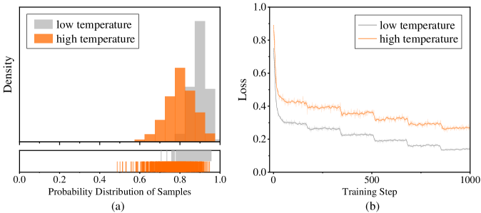
\n ## Charts: Probability Distribution and Loss vs. Training Step ### Overview The image presents two charts side-by-side. Chart (a) displays the probability distribution of samples for "low temperature" and "high temperature" settings, represented as histograms. Chart (b) shows the loss function value plotted against the training step, also for "low temperature" and "high temperature" settings, represented as lines. ### Components/Axes **Chart (a): Probability Distribution of Samples** * **X-axis:** Probability Distribution of Samples (ranging from approximately 0.0 to 1.0) * **Y-axis:** Density (no specific scale indicated, but values range from approximately 0 to 1) * **Legend:** * low temperature (represented by a light gray color) * high temperature (represented by an orange color) **Chart (b): Loss vs. Training Step** * **X-axis:** Training Step (ranging from 0 to 1000) * **Y-axis:** Loss (ranging from approximately 0.0 to 1.0) * **Legend:** * low temperature (represented by a light gray color) * high temperature (represented by an orange color) ### Detailed Analysis or Content Details **Chart (a): Probability Distribution of Samples** * **Low Temperature (Gray):** The distribution is heavily skewed towards higher probability values (approximately 0.7 to 1.0). The density is highest around 0.85, with a gradual decline towards lower probabilities. There is a small peak around 0.2. * **High Temperature (Orange):** The distribution is more spread out, with a peak around 0.65 and a significant tail extending towards lower probabilities (0.0 to 0.4). The density is lower overall compared to the low-temperature distribution. There are several small peaks between 0.4 and 0.7. **Chart (b): Loss vs. Training Step** * **Low Temperature (Gray):** The loss decreases rapidly from approximately 0.8 to around 0.15 within the first 200 training steps. After that, the loss continues to decrease, but at a much slower rate, with some plateaus and minor fluctuations. The final loss value at training step 1000 is approximately 0.1. * **High Temperature (Orange):** The loss also decreases initially, but not as rapidly as the low-temperature case. It starts at approximately 0.8 and reaches around 0.35 by training step 200. The loss then fluctuates more significantly, with several plateaus and increases, ending at a loss value of approximately 0.3 at training step 1000. ### Key Observations * The high-temperature setting results in a more diverse probability distribution (Chart a), while the low-temperature setting leads to a more concentrated distribution. * The low-temperature setting achieves a lower loss value (Chart b) and converges faster than the high-temperature setting. * The high-temperature setting exhibits more instability in the loss function during training, as evidenced by the fluctuations. ### Interpretation The charts likely represent the training process of a machine learning model, potentially a generative model. The "temperature" parameter controls the randomness of the model's output. * **Chart (a)** demonstrates that a higher temperature leads to a more uniform probability distribution, indicating greater exploration of the output space. Conversely, a lower temperature results in a more peaked distribution, favoring more probable outputs. * **Chart (b)** shows that a lower temperature leads to faster convergence and a lower final loss, suggesting that the model learns more efficiently when the output is less random. However, the higher temperature might be necessary for exploring a wider range of possibilities and avoiding local optima, even if it results in slower convergence and a higher loss. The difference in loss curves suggests a trade-off between exploration and exploitation. The low temperature prioritizes exploitation (refining existing knowledge), while the high temperature prioritizes exploration (discovering new possibilities). The optimal temperature setting would depend on the specific task and the desired balance between these two factors. The fluctuations in the high-temperature loss curve could indicate that the model is struggling to settle on a stable solution due to the increased randomness.