## Diagram: Neural Network Architectures - Deterministic vs. Probabilistic Weights
### Overview
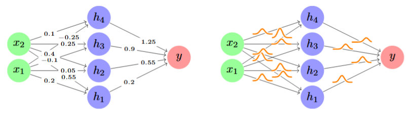
The image displays two side-by-side diagrams of a simple feedforward neural network with one hidden layer. The left diagram represents a standard network with deterministic, scalar weights on its connections. The right diagram represents a Bayesian or probabilistic neural network, where the weights are replaced by probability distributions (visualized as bell curves), indicating uncertainty in the parameter values.
### Components/Axes
**Common Structure (Both Diagrams):**
* **Input Layer (Left):** Two green circular nodes labeled `x1` (bottom) and `x2` (top).
* **Hidden Layer (Center):** Four blue circular nodes labeled `h1` (bottom), `h2`, `h3`, and `h4` (top).
* **Output Layer (Right):** One red circular node labeled `y`.
* **Connections:** Directed arrows (edges) flow from every input node to every hidden node, and from every hidden node to the output node, forming a fully connected network.
**Left Diagram - Deterministic Weights:**
* Each connection arrow is annotated with a specific numerical weight value.
* **Weights from Input to Hidden Layer:**
* From `x2`: to `h4` (0.1), to `h3` (-0.25), to `h2` (0.4), to `h1` (-0.1).
* From `x1`: to `h4` (0.05), to `h3` (0.55), to `h2` (0.2), to `h1` (0.2).
* **Weights from Hidden to Output Layer:**
* From `h4`: to `y` (1.25).
* From `h3`: to `y` (0.9).
* From `h2`: to `y` (0.55).
* From `h1`: to `y` (0.2).
**Right Diagram - Probabilistic Weights:**
* Each connection arrow is overlaid with an orange bell curve (Gaussian distribution symbol).
* No numerical values are present. The curves signify that each weight is not a single number but a distribution, representing a range of possible values with associated probabilities.
### Detailed Analysis
**Spatial Grounding & Component Isolation:**
1. **Header/Structure Region:** The overall layout is identical in both panels, establishing a direct visual comparison. The node colors (green=input, blue=hidden, red=output) are consistent.
2. **Main Chart/Data Region:**
* **Left Panel (Deterministic):** The data consists of 12 scalar weight values. The trend is simply the mapping of these fixed parameters. For example, the connection from `x2` to `h3` has a negative weight (-0.25), while from `x1` to `h3` is strongly positive (0.55).
* **Right Panel (Probabilistic):** The "data" is the presence of 12 distribution symbols. The visual trend is the replacement of every single number with a curve, indicating a shift from a single-point estimate to a full posterior distribution for each parameter.
3. **Footer/Label Region:** Node labels (`x1`, `x2`, `h1`-`h4`, `y`) are clearly placed inside or adjacent to their respective nodes in both diagrams.
### Key Observations
* **Direct One-to-One Correspondence:** Every connection with a numerical weight in the left diagram has a corresponding probability distribution curve in the exact same spatial position in the right diagram.
* **Visual Metaphor:** The orange curves are stylized Gaussian distributions, a common choice for weight priors/posteriors in Bayesian neural networks.
* **Complexity Contrast:** The left diagram is simple and concrete. The right diagram is more abstract, conveying increased model complexity and the incorporation of uncertainty.
* **No Outliers in Data:** The weight values on the left range from -0.25 to 1.25, with no extreme outliers. The distributions on the right are all depicted with similar shape and scale.
### Interpretation
This image is a pedagogical illustration contrasting two fundamental approaches to neural network modeling.
* **What it demonstrates:** It visually explains the core concept of a Bayesian Neural Network (BNN). In a traditional network (left), learning results in a single best estimate for each weight. In a BNN (right), learning results in a *distribution* for each weight, capturing the model's uncertainty about the true parameter value given the data.
* **Relationship between elements:** The side-by-side layout forces a direct comparison. The identical architecture (nodes and connections) highlights that the difference lies solely in the *nature of the weights*—deterministic scalars vs. probabilistic distributions.
* **Underlying significance:** The right diagram implies several advanced capabilities:
1. **Uncertainty Quantification:** The model can express how confident it is in its predictions by propagating weight uncertainty.
2. **Robustness:** Models with weight uncertainty are often less prone to overfitting.
3. **Bayesian Inference:** The distributions can be updated with new data using Bayes' theorem, moving from a prior to a posterior distribution.
* **Peircean Investigative Reading:** The image is an *icon* (resembling the structure of a neural network) that also functions as a *symbol* (using the established convention of a bell curve to represent a probability distribution). Its purpose is to create an immediate, intuitive understanding of a complex mathematical concept by leveraging visual analogy. The viewer is meant to infer that the "fuzzy" weights on the right lead to "fuzzier" but more honest predictions.