## Log-Log Plot of Gradient Updates vs. Dimension
### Overview
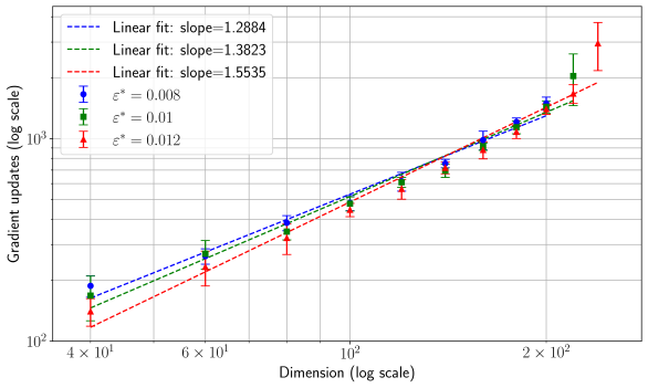
The image is a scientific scatter plot with error bars and linear regression fits, presented on a log-log scale. It illustrates the relationship between the dimension of a problem (x-axis) and the number of gradient updates required (y-axis) for three different values of a parameter denoted as ε* (epsilon star). The plot demonstrates a power-law relationship, as indicated by the linear trends on the logarithmic axes.
### Components/Axes
* **X-Axis:**
* **Label:** `Dimension (log scale)`
* **Scale:** Logarithmic.
* **Major Tick Marks:** `4 × 10¹`, `6 × 10¹`, `10²`, `2 × 10²`. These correspond to the numerical values 40, 60, 100, and 200.
* **Y-Axis:**
* **Label:** `Gradient updates (log scale)`
* **Scale:** Logarithmic.
* **Major Tick Marks:** `10²`, `10³`. These correspond to the numerical values 100 and 1000.
* **Legend (Located in the top-left corner):**
* The legend contains six entries, pairing data series symbols with their corresponding linear fit lines.
* **Data Series:**
1. Blue circle with error bars: `ε* = 0.008`
2. Green square with error bars: `ε* = 0.01`
3. Red triangle with error bars: `ε* = 0.012`
* **Linear Fit Lines:**
1. Blue dashed line: `Linear fit: slope=1.2884`
2. Green dashed line: `Linear fit: slope=1.3823`
3. Red dashed line: `Linear fit: slope=1.5535`
### Detailed Analysis
The plot shows three distinct data series, each following an upward linear trend on the log-log scale. This indicates a power-law relationship of the form `Gradient updates ∝ (Dimension)^slope`.
**Trend Verification:** All three data series (blue, green, red) show a clear upward slope from left to right, confirming that the number of gradient updates increases with dimension.
**Data Series and Approximate Points:**
1. **Blue Series (ε* = 0.008):**
* Trend: Slopes upward with the shallowest slope of the three fits (1.2884).
* Approximate Data Points (Dimension, Gradient updates):
* (40, ~150)
* (60, ~250)
* (100, ~450)
* (150, ~700)
* (200, ~1000)
2. **Green Series (ε* = 0.01):**
* Trend: Slopes upward with a moderate slope (1.3823).
* Approximate Data Points (Dimension, Gradient updates):
* (40, ~130)
* (60, ~220)
* (100, ~400)
* (150, ~650)
* (200, ~950)
3. **Red Series (ε* = 0.012):**
* Trend: Slopes upward with the steepest slope (1.5535).
* Approximate Data Points (Dimension, Gradient updates):
* (40, ~110)
* (60, ~180)
* (100, ~350)
* (150, ~600)
* (200, ~1200) - *Note: This final red point has a notably large error bar extending significantly above the trend line.*
**Error Bars:** All data points include vertical error bars, indicating variability or uncertainty in the measured "Gradient updates." The error bars generally increase in size with dimension, with the red series (ε* = 0.012) showing the largest uncertainty at the highest dimension (200).
### Key Observations
1. **Consistent Scaling Law:** All three conditions follow a clear power-law scaling, evidenced by the linear fits on the log-log plot.
2. **Slope Dependence on ε*:** The exponent (slope) of the power law increases with the parameter ε*. The relationship is: higher ε* leads to a steeper slope (1.2884 < 1.3823 < 1.5535).
3. **Crossover at Low Dimension:** At the lowest dimension (40), the order of required updates is inverted compared to higher dimensions: Blue (ε*=0.008) requires the *most* updates, while Red (ε*=0.012) requires the *fewest*. This order flips as dimension increases.
4. **Increasing Uncertainty:** The variability in the number of gradient updates (size of error bars) tends to grow with the problem dimension for all series.
### Interpretation
This plot likely comes from an optimization or machine learning context, analyzing how the computational cost (gradient updates) scales with the problem size (dimension) for different algorithmic settings (ε*).
* **What the data suggests:** The number of gradient updates needed to solve a problem scales as a power law with the problem's dimension. The exponent of this scaling law is not fixed but is controlled by the parameter ε*. A larger ε* results in a worse (steeper) scaling exponent, meaning the computational cost grows more rapidly with dimension.
* **Relationship between elements:** The parameter ε* acts as a tuning knob that trades off performance at low dimensions versus scalability. While a larger ε* (red) is more efficient for small problems (dimension ~40), it becomes less efficient than smaller ε* values for large-scale problems due to its steeper scaling. The crossover point appears to be around dimension 60-100.
* **Notable Anomalies:** The final red data point at dimension 200 is a potential outlier. Its central value lies above the fitted line, and its very large error bar suggests high instability or variance in the measurement for that specific condition (high ε*, high dimension). This could indicate the onset of a different regime or numerical challenges.
* **Underlying Implication:** For large-scale applications (high dimension), choosing a smaller ε* (e.g., 0.008) is crucial for better asymptotic performance, despite it being slightly less efficient for tiny problems. The analysis provides a quantitative basis for selecting algorithmic parameters based on the expected problem scale.