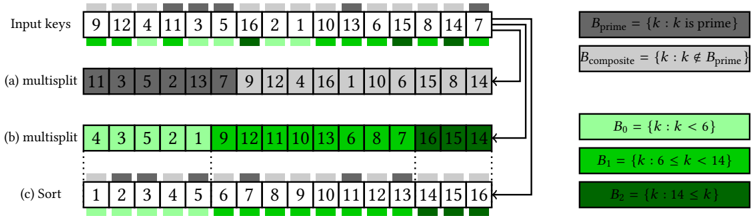
## Diagram: Multi-Key Sorting Algorithm Visualization
### Overview
The image is a technical diagram illustrating a multi-step sorting or partitioning algorithm applied to a set of integer keys from 1 to 16. The process uses two classification criteria: primality (prime vs. composite) and numerical range. The diagram shows the transformation of the input sequence through two "multisplit" stages and a final sort, with color-coding to indicate the classification of each number.
### Components/Axes
* **Main Structure:** Four horizontal rows of numbered boxes, labeled sequentially:
* **Input keys:** The initial, unsorted sequence.
* **(a) multisplit:** The first partitioning step.
* **(b) multisplit:** The second partitioning/sorting step.
* **(c) Sort:** The final, fully sorted sequence.
* **Legend (Right Side):** Defines the color-coding scheme.
* **Gray Scale (Prime/Composite):**
* `B_prime = {k : k is prime}` (Light gray box)
* `B_composite = {k : k ∉ B_prime}` (Dark gray box)
* **Green Scale (Value Ranges):**
* `B₀ = {k : k < 6}` (Light green box)
* `B₁ = {k : 6 ≤ k < 14}` (Medium green box)
* `B₂ = {k : 14 ≤ k}` (Dark green box)
* **Flow Arrows:** Black arrows connect the rows, indicating the progression from "Input keys" to "(a) multisplit," then to "(b) multisplit," and finally to "(c) Sort."
### Detailed Analysis
**1. Input Keys Sequence & Classification:**
The initial sequence is: `9, 12, 4, 11, 3, 5, 16, 2, 1, 10, 13, 6, 15, 8, 14, 7`.
* **Color/Classification Mapping:**
* **Light Green (B₀: k < 6):** 9, 4, 1
* **Medium Green (B₁: 6 ≤ k < 14):** 12, 10, 13, 6, 8
* **Dark Green (B₂: 14 ≤ k):** 16, 15, 14
* **Gray (Primes):** 11, 3, 5, 2, 7 (Note: 13 is prime but is colored medium green, indicating the primary visual classification in the diagram is by value range, not primality).
**2. Step (a) multisplit:**
The sequence becomes: `11, 3, 5, 2, 13, 7, 9, 12, 4, 16, 1, 10, 6, 15, 8, 14`.
* **Trend/Observation:** The first six positions are occupied by numbers colored gray (primes: 11, 3, 5, 2, 7) and one medium green (13, a prime). The remaining ten positions contain the non-prime numbers, colored in green shades. This suggests the first split separates primes from composites.
**3. Step (b) multisplit:**
The sequence becomes: `4, 3, 5, 2, 1, 9, 12, 11, 10, 13, 6, 8, 7, 16, 15, 14`.
* **Trend/Observation:** The sequence is now partially sorted. The first five numbers are primarily from B₀ (light green: 4, 1, 9) interspersed with some primes (gray: 3, 5, 2). The middle section contains numbers from B₁ (medium green: 12, 10, 13, 6, 8) and primes (gray: 11, 7). The final three are from B₂ (dark green: 16, 15, 14). This indicates a secondary partitioning based on value ranges within the groups established in step (a).
**4. Step (c) Sort (Final Output):**
The sequence is fully sorted in ascending order: `1, 2, 3, 4, 5, 6, 7, 8, 9, 10, 11, 12, 13, 14, 15, 16`.
* **Color Pattern in Sorted Order:** The colors now follow a clear, non-overlapping pattern based on the value ranges (B₀, B₁, B₂), with primes (gray) appearing within their respective numerical ranges. For example, 2, 3, 5, 7, 11, 13 are gray but are placed in their correct sorted positions among the green-shaded numbers.
### Key Observations
1. **Dual Classification:** The algorithm uses two independent properties of the numbers: whether they are prime (a mathematical property) and their magnitude (a numerical property).
2. **Visual Priority:** While the legend defines both gray (prime) and green (range) schemes, the diagram's primary visual encoding in the intermediate steps appears to be the green value-range scheme. The gray color is used to highlight primes within those ranges.
3. **Progressive Sorting:** The process moves from a completely unsorted state, to a state grouped by primality, to a state grouped by value range within primality groups, and finally to a fully sorted sequence.
4. **Spatial Layout:** The legend is positioned to the right of the main diagram. The four processing steps are stacked vertically, with flow arrows clearly indicating the sequence of operations from top to bottom.
### Interpretation
This diagram serves as an educational visualization of a **multi-key sorting algorithm**. It demonstrates how complex sorting can be broken down into simpler, sequential partitioning steps based on different attributes of the data.
* **What it Suggests:** The data suggests that sorting can be achieved efficiently by applying a series of "multisplit" operations, each refining the order based on a specific criterion (first primality, then magnitude). This is analogous to algorithms like Radix Sort or Bucket Sort, which sort data in passes based on individual digits or ranges.
* **Relationship Between Elements:** The "Input keys" are the raw data. Steps (a) and (b) are the core algorithmic operations, transforming the data's organization. The "Sort" row is the final, desired output. The legend provides the key to understanding the state of the data at each intermediate step.
* **Notable Insight:** The final sorted sequence shows that the two classification schemes (prime/composite and value range) are orthogonal. A number's primality does not affect its final sorted position relative to other numbers; only its numerical value does. The color in the final row simply annotates the properties of the already-sorted numbers. The algorithm's intermediate steps, however, leverage these properties to achieve the sort.