## Line Chart: L0 over Training Steps
### Overview
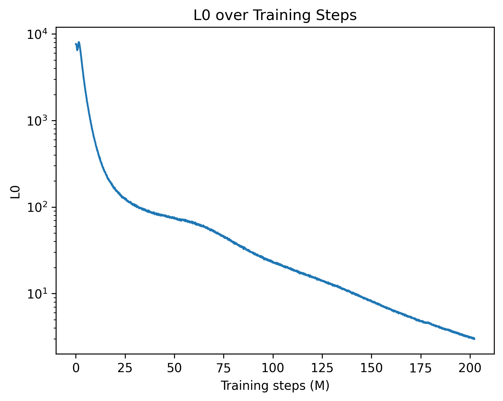
This image is a line chart depicting the progression of a metric labeled "L0" over a period of 200 million "Training steps". The chart illustrates a rapid initial decline in the L0 metric, followed by a slower, continuous exponential decay.
### Components/Axes
* **Header (Top Center):** The title of the chart is "L0 over Training Steps".
* **X-Axis (Bottom):**
* **Label:** "Training steps (M)" positioned at the bottom center. The "(M)" likely denotes millions.
* **Scale:** Linear.
* **Markers:** Major tick marks are placed at intervals of 25, specifically labeled at: 0, 25, 50, 75, 100, 125, 150, 175, and 200.
* **Y-Axis (Left):**
* **Label:** "L0" positioned vertically along the left edge.
* **Scale:** Logarithmic (base 10).
* **Markers:** Major tick marks are labeled at $10^1$, $10^2$, $10^3$, and $10^4$. Minor tick marks are visible between these major powers of 10, indicating the logarithmic progression.
* **Data Series:** A single, solid blue line representing the L0 value.
* **Legend:** There is no legend present, as there is only one data series.
### Detailed Analysis
**Trend Verification:**
The blue line begins near the top-left of the chart area, just below the $10^4$ mark. It exhibits a very steep, almost vertical downward slope during the initial training steps. Around the 25M step mark, the rate of descent slows significantly, creating a "shoulder" or inflection point in the curve between 25M and 75M steps. After 75M steps, the line settles into a steady, near-linear downward slope on this logarithmic scale, indicating a consistent exponential decay until the end of the recorded steps. The line is slightly jagged throughout, indicating minor step-to-step variance rather than a perfectly smoothed average.
**Approximate Data Points (with uncertainty due to log scale):**
* **X = 0:** The line starts with a tiny spike, peaking just below $10^4$ (approximately 8,000 - 9,000).
* **X = 10:** The value drops precipitously by a full order of magnitude to approximately $10^3$ (1,000).
* **X = 25:** The steep drop begins to level out, with the value sitting slightly above $10^2$ (approximately 120 - 150).
* **X = 50:** The curve flattens noticeably here, with the value dropping just below $10^2$ (approximately 80 - 90).
* **X = 75:** The steady decay phase begins, with the value at approximately 50.
* **X = 100:** The value is approximately 25 - 30.
* **X = 125:** The value is approximately 15.
* **X = 150:** The line crosses below the $10^1$ major tick mark, sitting at approximately 8 - 9.
* **X = 175:** The value is approximately 5.
* **X = 200:** The chart concludes with the L0 value at its lowest point, approximately 3.
### Key Observations
1. **Massive Initial Reduction:** The most significant observation is the reduction of the L0 metric by nearly two orders of magnitude (from ~8000 to ~100) within the first 12.5% of the training process (0 to 25M steps).
2. **Phase Transition:** The distinct change in the slope between 25M and 75M steps suggests a shift in the training dynamics.
3. **Diminishing Returns:** While the metric continues to improve (decrease) all the way to 200M steps, the absolute reduction in the final 100M steps (dropping from ~30 to ~3) is minuscule compared to the first 25M steps, though it remains significant on a relative/logarithmic basis.
### Interpretation
In the context of machine learning and neural network training, this chart represents a classic loss or penalty curve.
* **What is L0?** While "L0" can sometimes refer to the L0-norm (a measure of sparsity counting non-zero elements), true L0 is non-differentiable. In modern deep learning, "L0" often refers to a continuous approximation of the L0 penalty (e.g., L0 regularization used to encourage sparse neural networks) or a specific component of a loss function.
* **Training Dynamics:** The graph demonstrates that the model rapidly optimizes the most obvious or impactful parameters early in the training run (the steep drop). The "shoulder" around 50M steps could indicate the model escaping a local minimum, a scheduled change in the learning rate, or a transition from learning broad features to fine-tuning complex, subtle patterns.
* **Reading Between the Lines (Peircean Investigative):** The choice of a logarithmic Y-axis is deliberate and necessary. If plotted on a linear scale, the curve after 25M steps would look like a flat line at zero, obscuring the fact that the model is still actively learning and improving. The slight, high-frequency jaggedness of the blue line implies that this data is plotted at a high resolution (perhaps every few hundred or thousand steps) rather than being heavily smoothed across entire epochs, revealing the inherent stochastic noise of batch-based gradient descent. The fact that the curve is still trending downward at 200M steps suggests that the model has not yet fully converged and could potentially benefit from further training, albeit at a very slow rate of absolute improvement.