## Line Chart: L0 over Training Steps
### Overview
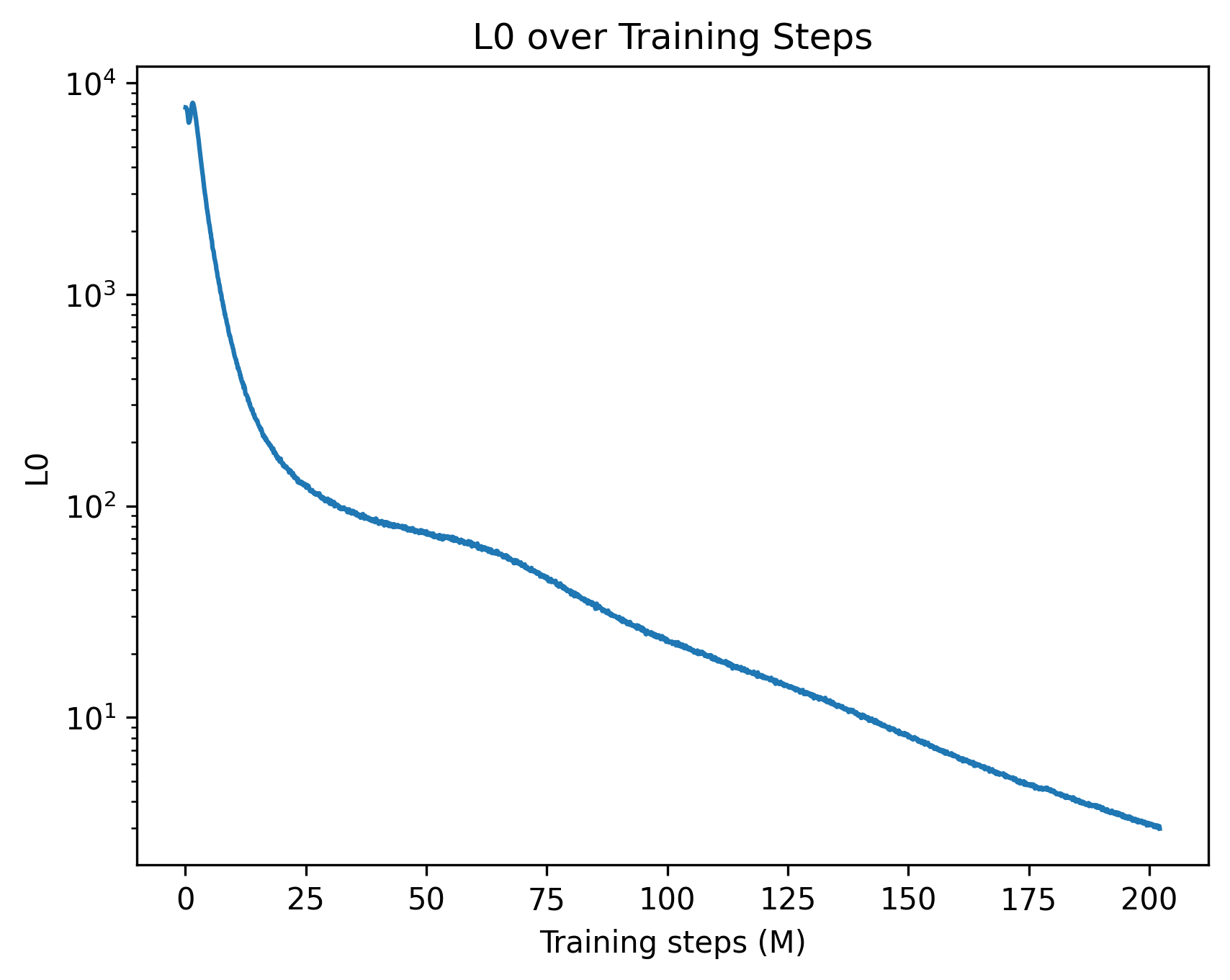
The image displays a single-line chart plotting a metric labeled "L0" against "Training steps (M)". The chart uses a logarithmic scale for the vertical axis (y-axis) and a linear scale for the horizontal axis (x-axis). The data shows a clear, continuous downward trend, indicating that the L0 value decreases as the number of training steps increases.
### Components/Axes
* **Chart Title:** "L0 over Training Steps" (centered at the top).
* **Y-Axis:**
* **Label:** "L0" (positioned vertically on the left side).
* **Scale:** Logarithmic (base 10).
* **Major Tick Marks & Labels:** `10^1` (10), `10^2` (100), `10^3` (1000), `10^4` (10000). The axis spans from just below 10^1 to just above 10^4.
* **X-Axis:**
* **Label:** "Training steps (M)" (centered at the bottom). The "(M)" likely denotes "Millions".
* **Scale:** Linear.
* **Major Tick Marks & Labels:** 0, 25, 50, 75, 100, 125, 150, 175, 200. The axis spans from 0 to 200 million steps.
* **Data Series:** A single, solid blue line representing the L0 metric over time. There is no legend, as only one series is present.
### Detailed Analysis
**Trend Verification:** The blue line exhibits a steep, near-vertical descent at the beginning of training, which then transitions into a progressively shallower, but still consistent, downward slope for the remainder of the charted steps.
**Approximate Data Points & Trend:**
* **At Step 0 (Start):** The line originates at a very high L0 value, approximately **8,000** (just below the 10^4 mark).
* **Initial Phase (0 to ~25M steps):** The line plummets dramatically. By step 25M, the L0 value has fallen to approximately **200** (slightly above the 10^2 mark). This represents a reduction of roughly 97.5% from the starting value.
* **Middle Phase (~25M to ~100M steps):** The rate of decrease slows but remains steady. The line passes through:
* ~50M steps: L0 ≈ **80**
* ~75M steps: L0 ≈ **40**
* ~100M steps: L0 ≈ **20** (aligning with the 10^1.3 region).
* **Late Phase (~100M to 200M steps):** The decline continues at a roughly constant, shallow slope on the log-linear plot. The line ends at 200M steps with an L0 value of approximately **4** (visibly below the 10^1 mark).
### Key Observations
1. **Logarithmic Scale Impact:** The use of a log scale on the y-axis compresses the visual representation of the massive initial drop and expands the view of the later, smaller improvements. On a linear scale, the curve would appear as an almost immediate drop followed by a long, flat tail.
2. **Two-Phase Learning:** The curve suggests two distinct phases of improvement: a rapid, initial "learning burst" followed by a prolonged period of gradual refinement.
3. **Consistent Improvement:** There are no visible plateaus, spikes, or reversals in the trend. The L0 metric improves (decreases) consistently throughout the entire 200 million training steps shown.
4. **Magnitude of Change:** The total improvement over the charted period is immense, spanning over three orders of magnitude (from ~8,000 to ~4).
### Interpretation
This chart is characteristic of a loss function or error metric (where "L0" likely stands for "Loss at stage 0" or a primary loss component) during the training of a machine learning model, particularly a neural network.
* **What the Data Suggests:** The model is successfully learning from the data. The steep initial drop indicates it is quickly grasping the most obvious patterns. The continued, slower decline shows it is fine-tuning its parameters to capture more subtle nuances, a process that yields diminishing returns per step but is crucial for high performance.
* **Relationship Between Elements:** The x-axis (training steps) is the independent variable representing computational effort. The y-axis (L0) is the dependent variable representing model performance (lower is better). The curve maps the efficiency of the training process.
* **Notable Implications:** The lack of a plateau by 200M steps suggests that further training might still yield (small) improvements, though the cost-benefit ratio is changing. The smoothness of the curve implies a stable training process with well-tuned hyperparameters (like learning rate). An investigator would use this plot to diagnose training health, decide when to stop training, and compare the efficiency of different model architectures or training algorithms.