## Chart Type: Comparative Line Graphs
### Overview
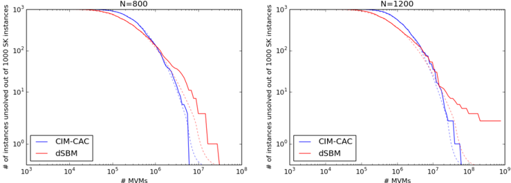
The image presents two line graphs comparing the performance of two algorithms, CIM-CAC and dSBM, in solving a set of instances. The graphs show the number of instances unsolved out of 1000 SK instances as a function of the number of MVMs (Million Vector Multiplications) required. The left graph corresponds to a dataset with N=800, while the right graph corresponds to N=1200. Both graphs use a log-log scale.
### Components/Axes
* **X-axis (horizontal):** "# MVMs" (Number of Million Vector Multiplications). Logarithmic scale, ranging from 10^3 to 10^8 for N=800, and 10^3 to 10^9 for N=1200.
* **Y-axis (vertical):** "# of instances unsolved out of 1000 SK instances". Logarithmic scale, ranging from 10^0 to 10^3.
* **Titles:** "N=800" (left graph), "N=1200" (right graph).
* **Legend (bottom-left of each graph):**
* Blue line: CIM-CAC
* Red line: dSBM
### Detailed Analysis
**Left Graph (N=800):**
* **CIM-CAC (Blue):** The line starts near 10^3 unsolved instances at 10^3 MVMs. It slopes downward, indicating that as the number of MVMs increases, the number of unsolved instances decreases. The line reaches approximately 1 unsolved instance around 10^7 MVMs.
* (10^3, 10^3)
* (10^4, ~300)
* (10^5, ~100)
* (10^6, ~20)
* (10^7, ~1)
* **dSBM (Red):** Similar to CIM-CAC, the line starts near 10^3 unsolved instances at 10^3 MVMs and slopes downward. However, it appears to decrease more slowly than CIM-CAC initially. The line reaches approximately 1 unsolved instance around 10^7 MVMs.
* (10^3, 10^3)
* (10^4, ~400)
* (10^5, ~100)
* (10^6, ~30)
* (10^7, ~2)
**Right Graph (N=1200):**
* **CIM-CAC (Blue):** The line starts near 10^3 unsolved instances at 10^3 MVMs. It slopes downward, indicating that as the number of MVMs increases, the number of unsolved instances decreases. The line reaches approximately 1 unsolved instance around 10^8 MVMs.
* (10^3, 10^3)
* (10^4, ~400)
* (10^5, ~100)
* (10^6, ~20)
* (10^7, ~2)
* (10^8, ~1)
* **dSBM (Red):** Similar to CIM-CAC, the line starts near 10^3 unsolved instances at 10^3 MVMs and slopes downward. However, it appears to decrease more slowly than CIM-CAC initially. The line reaches approximately 1 unsolved instance around 10^8 MVMs.
* (10^3, 10^3)
* (10^4, ~500)
* (10^5, ~100)
* (10^6, ~30)
* (10^7, ~5)
* (10^8, ~2)
### Key Observations
* Both algorithms, CIM-CAC and dSBM, show a decrease in the number of unsolved instances as the number of MVMs increases.
* For N=800, CIM-CAC appears to perform slightly better than dSBM, reaching lower unsolved instance counts for a given number of MVMs.
* For N=1200, the difference in performance between CIM-CAC and dSBM is less pronounced, especially at higher MVM counts.
* The N=1200 graphs show that more MVMs are required to solve the same number of instances compared to N=800.
### Interpretation
The graphs illustrate the trade-off between computational effort (MVMs) and the number of unsolved instances for two different algorithms. The downward slope of the lines indicates that increasing the computational effort generally leads to solving more instances. The comparison between CIM-CAC and dSBM suggests that CIM-CAC may be more efficient for smaller datasets (N=800), but the performance difference diminishes as the dataset size increases (N=1200). The shift of the curves to the right for N=1200 indicates that larger datasets require more computational resources to achieve the same level of problem-solving. The dashed lines likely represent some form of confidence interval or variance in the data.