## Comparative Performance Chart: CIM-CAC vs. dSBM on SK Instances
### Overview
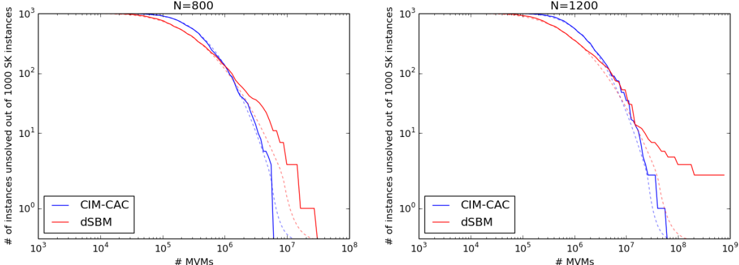
The image displays two side-by-side log-log plots comparing the performance of two algorithms, **CIM-CAC** (blue line) and **dSBM** (red line), on Sherrington-Kirkpatrick (SK) spin-glass instances. The plots show the number of unsolved instances as a function of computational effort, measured in Matrix-Vector Multiplications (MVMs). The left plot is for problem size **N=800**, and the right plot is for **N=1200**. Each plot tracks the progress of solving a set of **1000 SK instances**.
### Components/Axes
* **Chart Type:** Two side-by-side log-log line charts.
* **Titles:**
* Left Chart: `N=800`
* Right Chart: `N=1200`
* **Y-Axis (Both Charts):**
* **Label:** `# of instances unsolved out of 1000 SK instances`
* **Scale:** Logarithmic, ranging from `10^0` (1) to `10^3` (1000).
* **Markers:** Major ticks at `10^0`, `10^1`, `10^2`, `10^3`.
* **X-Axis (Both Charts):**
* **Label:** `# MVMs`
* **Scale:** Logarithmic.
* **Left Chart (N=800) Range:** Approximately `10^3` to `10^8`.
* **Right Chart (N=1200) Range:** Approximately `10^4` to `10^9`.
* **Legend (Bottom-Left of each plot):**
* **Blue Line:** `CIM-CAC`
* **Red Line:** `dSBM`
* **Data Series:** Two lines per chart, corresponding to the legend.
### Detailed Analysis
**Left Chart (N=800):**
* **Trend Verification:** Both lines start at the top-left (1000 unsolved instances at low MVMs) and slope downward to the right, indicating that more instances are solved as computational effort (MVMs) increases. The blue line (CIM-CAC) descends more steeply than the red line (dSBM).
* **Data Points & Values (Approximate):**
* At ~`10^5` MVMs: Both algorithms still have nearly 1000 instances unsolved.
* At ~`10^6` MVMs:
* CIM-CAC (Blue): ~100 instances unsolved.
* dSBM (Red): ~200 instances unsolved.
* At ~`5*10^6` MVMs:
* CIM-CAC (Blue): Drops sharply to near 0 unsolved instances.
* dSBM (Red): ~10 instances unsolved.
* At ~`10^7` MVMs:
* CIM-CAC (Blue): 0 instances unsolved (line ends).
* dSBM (Red): ~1 instance unsolved.
* The dSBM (Red) line shows a final step down to 0 unsolved instances just before `10^8` MVMs.
**Right Chart (N=1200):**
* **Trend Verification:** Similar initial downward trend for both. The performance gap between the two algorithms is more pronounced here. The blue line (CIM-CAC) again descends steeply, while the red line (dSBM) declines more gradually and exhibits a clear plateau.
* **Data Points & Values (Approximate):**
* At ~`10^6` MVMs: Both algorithms still have nearly 1000 instances unsolved.
* At ~`10^7` MVMs:
* CIM-CAC (Blue): ~100 instances unsolved.
* dSBM (Red): ~300 instances unsolved.
* At ~`5*10^7` MVMs:
* CIM-CAC (Blue): ~1 instance unsolved.
* dSBM (Red): ~10 instances unsolved.
* At ~`10^8` MVMs:
* CIM-CAC (Blue): 0 instances unsolved (line ends).
* dSBM (Red): Plateaus at approximately 2-3 instances unsolved. The line remains flat from ~`10^8` to `10^9` MVMs, indicating these few instances are not solved with additional computation within the tested range.
### Key Observations
1. **Consistent Superiority of CIM-CAC:** In both problem sizes (N=800 and N=1200), the CIM-CAC algorithm (blue) solves all 1000 instances with significantly fewer MVMs than the dSBM algorithm (red).
2. **Impact of Problem Size:** The performance gap widens as the problem size increases from N=800 to N=1200. For N=1200, dSBM fails to solve a small subset of instances (~2-3) even after `10^9` MVMs, whereas CIM-CAC solves all instances by `10^8` MVMs.
3. **Plateau in dSBM (N=1200):** The red line in the right chart shows a distinct plateau starting around `10^8` MVMs, suggesting a subset of "hard" instances for the dSBM algorithm at this larger problem size.
4. **Steep Descent of CIM-CAC:** The blue line in both charts exhibits a very steep, almost vertical drop in the final phase, indicating that once CIM-CAC begins solving the remaining instances, it does so very rapidly in terms of additional MVMs.
### Interpretation
This data demonstrates a clear and significant performance advantage for the **CIM-CAC** algorithm over the **dSBM** algorithm on the tested SK spin-glass optimization problem. The key metric is computational efficiency: CIM-CAC requires approximately **one order of magnitude fewer Matrix-Vector Multiplications** to solve the same set of problem instances.
The relationship between the elements is a direct comparison of algorithmic efficiency. The x-axis (# MVMs) represents computational cost, and the y-axis (# unsolved instances) represents progress. A steeper, leftmost curve is better.
**Notable Anomaly/Outlier:** The plateau in the dSBM curve for N=1200 is the most significant outlier. It indicates the existence of a specific class of problem instances within the SK model that are particularly resistant to the dSBM solution method at scale, while remaining tractable for CIM-CAC. This suggests a fundamental difference in how the two algorithms navigate the problem's energy landscape.
**Why it matters:** For practical applications involving complex optimization (like those modeled by SK spin glasses), choosing CIM-CAC over dSBM could lead to dramatic reductions in computation time and resource usage, especially for larger, more realistic problem sizes. The results imply CIM-CAC has a more effective strategy for avoiding or escaping the local minima that appear to stall dSBM.