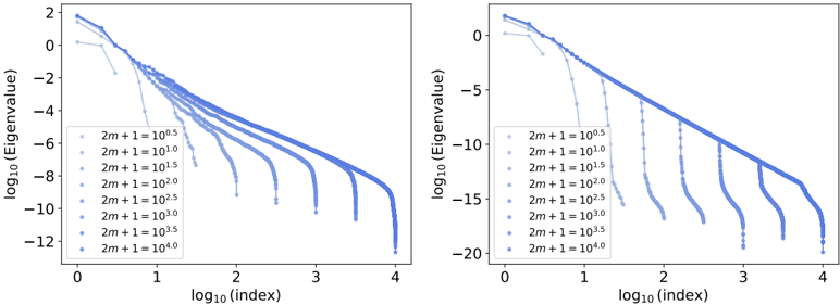
## Line Graphs: Eigenvalue Trends vs. Index (log10 Scale) ### Overview The image contains two side-by-side line graphs comparing the logarithmic scale of eigenvalues (log₁₀(Eigenvalue)) against the logarithmic scale of an index (log₁₀(index)). Each graph displays multiple data series, differentiated by the parameter "2m + 1" (e.g., 10⁰.⁵, 10¹.⁰, ..., 10⁴.⁰). The left graph shows a steeper decline in eigenvalues for higher "2m + 1" values, while the right graph exhibits a more gradual decline with secondary drops. --- ### Components/Axes - **X-axis (log₁₀(index))**: Ranges from 0 to 4 (log₁₀ scale), representing the index values from 10⁰ to 10⁴. - **Y-axis (log₁₀(Eigenvalue))**: Ranges from 0 to -20 (log₁₀ scale), representing eigenvalues from 1 to 10⁻²⁰. - **Legends**: - **Left Graph**: Legend positioned at the bottom-left, listing "2m + 1 = 10⁰.⁵" to "2m + 1 = 10⁴.⁰" with corresponding line styles. - **Right Graph**: Legend positioned at the bottom-right, listing the same "2m + 1" values with matching line styles. --- ### Detailed Analysis #### Left Graph - **Data Series**: - Lines for "2m + 1 = 10⁰.⁵" to "2m + 1 = 10⁴.⁰" are plotted. - All lines start near 0 on the y-axis and decline sharply as the index increases. - Higher "2m + 1" values (e.g., 10³.⁰, 10⁴.⁰) show steeper slopes, indicating faster eigenvalue decay. - Some lines (e.g., "2m + 1 = 10².⁵") exhibit a secondary drop near log₁₀(index) ≈ 2.5. #### Right Graph - **Data Series**: - Lines for "2m + 1 = 10⁰.⁵" to "2m + 1 = 10⁴.⁰" are plotted. - Lines start near 0 and decline gradually compared to the left graph. - Secondary drops occur at log₁₀(index) ≈ 1.5, 2.5, and 3.5 for higher "2m + 1" values (e.g., 10³.⁰, 10⁴.⁰). - The decline is less steep overall, with eigenvalues remaining higher for longer index ranges. --- ### Key Observations 1. **Eigenvalue Decay**: - Higher "2m + 1" values correlate with faster eigenvalue decay (left graph) or more pronounced secondary drops (right graph). - The right graph shows eigenvalues persisting at higher magnitudes for longer index ranges. 2. **Secondary Drops**: - Observed in both graphs but more frequent and pronounced in the right graph, suggesting threshold effects or phase transitions. 3. **Scale Sensitivity**: - Logarithmic scaling emphasizes exponential trends, making small differences in "2m + 1" values visually significant. --- ### Interpretation The data suggests that the parameter "2m + 1" critically influences the eigenvalue behavior of a system. In the left graph, the steeper decay implies a more sensitive or unstable system for higher "2m + 1" values. The right graph’s secondary drops may indicate discrete transitions or resonances at specific index thresholds. The logarithmic scaling highlights exponential relationships, which could relate to phenomena like damping, resonance, or stability thresholds in physical or mathematical systems. The divergence in trends between the two graphs might reflect different modeling assumptions or experimental conditions.