## Chart: Eigenvalue and Effective Dimension Plots
### Overview
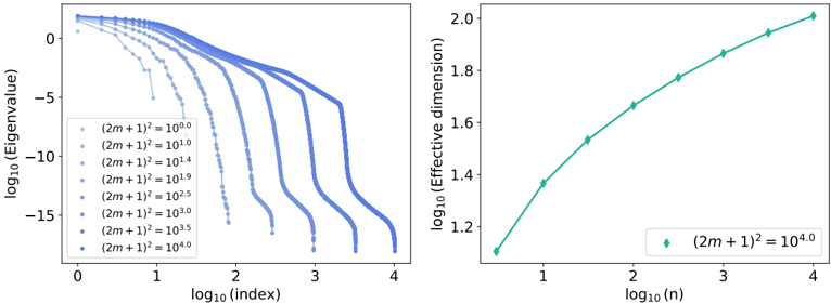
The image presents two plots side-by-side. The left plot shows the logarithm base 10 of the eigenvalue versus the logarithm base 10 of the index for different values of (2m+1)^2. The right plot shows the logarithm base 10 of the effective dimension versus the logarithm base 10 of n for (2m+1)^2 = 10^4.0.
### Components/Axes
**Left Plot:**
* **X-axis:** log₁₀(index), ranging from 0 to 4.
* **Y-axis:** log₁₀(Eigenvalue), ranging from -15 to 0.
* **Legend (top-left):**
* (2m+1)² = 10⁰⁰ (lightest blue)
* (2m+1)² = 10¹⁰ (lighter blue)
* (2m+1)² = 10¹⁴ (light blue)
* (2m+1)² = 10¹⁹ (mid-blue)
* (2m+1)² = 10².⁵ (darker blue)
* (2m+1)² = 10³.⁰ (dark blue)
* (2m+1)² = 10³.⁵ (darkest blue)
* (2m+1)² = 10⁴⁰ (darkest blue)
**Right Plot:**
* **X-axis:** log₁₀(n), ranging from 1 to 4.
* **Y-axis:** log₁₀(Effective dimension), ranging from 1.0 to 2.0.
* **Legend (bottom):**
* (2m+1)² = 10⁴⁰ (teal)
### Detailed Analysis
**Left Plot (Eigenvalue vs. Index):**
Each line represents a different value of (2m+1)². All lines show a general downward trend, indicating that the eigenvalue decreases as the index increases. The lines start at approximately log₁₀(Eigenvalue) = 0 and then decrease. The rate of decrease varies, with the lines for smaller values of (2m+1)² decreasing more rapidly initially. Each line plateaus at a different point on the x-axis, with the plateau point shifting to the right as (2m+1)² increases.
* **(2m+1)² = 10⁰⁰ (lightest blue):** Starts at approximately (0, 0) and rapidly decreases to approximately (1, -15).
* **(2m+1)² = 10¹⁰ (lighter blue):** Starts at approximately (0, 0) and decreases to approximately (1.5, -15).
* **(2m+1)² = 10¹⁴ (light blue):** Starts at approximately (0, 0) and decreases to approximately (2, -15).
* **(2m+1)² = 10¹⁹ (mid-blue):** Starts at approximately (0, 0) and decreases to approximately (2.5, -15).
* **(2m+1)² = 10².⁵ (darker blue):** Starts at approximately (0, 0) and decreases to approximately (3, -15).
* **(2m+1)² = 10³.⁰ (dark blue):** Starts at approximately (0, 0) and decreases to approximately (3.2, -15).
* **(2m+1)² = 10³.⁵ (darkest blue):** Starts at approximately (0, 0) and decreases to approximately (3.5, -15).
* **(2m+1)² = 10⁴⁰ (darkest blue):** Starts at approximately (0, 0) and decreases to approximately (3.8, -15).
**Right Plot (Effective Dimension vs. n):**
The teal line represents (2m+1)² = 10⁴⁰. The line slopes upward, indicating that the effective dimension increases as n increases.
* At log₁₀(n) = 1, log₁₀(Effective dimension) ≈ 1.1.
* At log₁₀(n) = 2, log₁₀(Effective dimension) ≈ 1.5.
* At log₁₀(n) = 3, log₁₀(Effective dimension) ≈ 1.8.
* At log₁₀(n) = 4, log₁₀(Effective dimension) ≈ 1.95.
### Key Observations
* In the left plot, as (2m+1)² increases, the eigenvalues decay more slowly with increasing index.
* In the right plot, the effective dimension increases with n, but the rate of increase slows down as n increases.
### Interpretation
The left plot illustrates how the eigenvalue spectrum changes with different values of (2m+1)². The slower decay of eigenvalues for larger (2m+1)² suggests a higher effective dimensionality or complexity in the system being analyzed. The right plot shows that the effective dimension grows with n, but the diminishing rate of increase suggests a saturation effect, where the effective dimension approaches a limit as n becomes very large. The plots together suggest that increasing (2m+1)² leads to a more complex system with a higher effective dimension, and that the effective dimension is related to the index n.