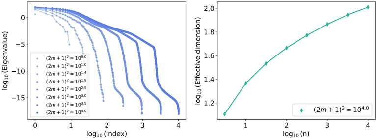
## [Chart Type]: Dual-Panel Scientific Plot ### Overview The image contains two separate but related scientific plots presented side-by-side. Both are line graphs with logarithmic axes, analyzing properties related to a parameter `(2m+1)^2`. The left panel shows the decay of eigenvalues across an index, while the right panel shows the growth of an "Effective dimension" with respect to a variable `n`. The plots use a consistent color scheme and mathematical notation. ### Components/Axes **Left Plot:** * **Title:** None visible. * **Y-axis:** Label is `log10(Eigenvalue)`. Scale ranges from approximately -15 to 0, with major tick marks at -15, -10, -5, and 0. * **X-axis:** Label is `log10(index)`. Scale ranges from 0 to 4, with major tick marks at 0, 1, 2, 3, and 4. * **Legend:** Located in the bottom-left corner. It lists 9 data series, each corresponding to a different value of `(2m+1)^2`. The entries are: * `(2m+1)^2 = 10^{0.0}` (lightest blue) * `(2m+1)^2 = 10^{0.5}` * `(2m+1)^2 = 10^{1.0}` * `(2m+1)^2 = 10^{1.5}` * `(2m+1)^2 = 10^{2.0}` * `(2m+1)^2 = 10^{2.5}` * `(2m+1)^2 = 10^{3.0}` * `(2m+1)^2 = 10^{3.5}` * `(2m+1)^2 = 10^{4.0}` (darkest blue) * **Data Series:** 9 distinct curves, each plotted with a unique shade of blue corresponding to the legend. The color gradient progresses from light to dark as the exponent in `(2m+1)^2` increases. **Right Plot:** * **Title:** None visible. * **Y-axis:** Label is `log10(Effective dimension)`. Scale ranges from approximately 1.1 to 2.0, with major tick marks at 1.2, 1.4, 1.6, 1.8, and 2.0. * **X-axis:** Label is `log10(n)`. Scale ranges from approximately 0.5 to 4, with major tick marks at 1, 2, 3, and 4. * **Legend:** Located in the bottom-right corner. It contains a single entry: * `(2m+1)^2 = 10^{4.0}` (teal color with diamond marker) * **Data Series:** A single curve plotted with a teal line and diamond-shaped markers. ### Detailed Analysis **Left Plot (Eigenvalue Spectrum):** * **Trend Verification:** All curves exhibit a similar downward-sloping trend. They start at a high `log10(Eigenvalue)` (near 0) for low `log10(index)` and decay towards very low values (approaching -15) as the index increases. The decay is not linear; it appears to have an initial slower decline followed by a steeper drop-off. * **Data Point Extraction (Approximate):** * For the series `(2m+1)^2 = 10^{0.0}` (lightest blue): The curve starts near (0, 0) and drops off most rapidly, reaching `log10(Eigenvalue) ≈ -15` by `log10(index) ≈ 1.5`. * For the series `(2m+1)^2 = 10^{4.0}` (darkest blue): The curve starts near (0, 0) and decays the slowest, maintaining a `log10(Eigenvalue) > -5` until `log10(index) ≈ 3`, before dropping sharply. * **General Pattern:** As the parameter `(2m+1)^2` increases (moving from light to dark blue curves), the eigenvalue spectrum decays more slowly. The "knee" of the curve, where the decay accelerates, shifts to the right (higher index) for larger parameter values. **Right Plot (Effective Dimension):** * **Trend Verification:** The single curve shows a clear upward-sloping, concave-down trend. The `log10(Effective dimension)` increases with `log10(n)`, but the rate of increase slows down. * **Data Point Extraction (Approximate):** * At `log10(n) ≈ 0.5`, `log10(Effective dimension) ≈ 1.1`. * At `log10(n) = 1.0`, `log10(Effective dimension) ≈ 1.38`. * At `log10(n) = 2.0`, `log10(Effective dimension) ≈ 1.67`. * At `log10(n) = 3.0`, `log10(Effective dimension) ≈ 1.86`. * At `log10(n) = 4.0`, `log10(Effective dimension) ≈ 2.0`. * The relationship appears to be sub-linear on this log-log scale, suggesting the effective dimension grows as a power law of `n` with an exponent less than 1. ### Key Observations 1. **Parameter Dependence (Left Plot):** The decay rate of the eigenvalue spectrum is strongly controlled by the parameter `(2m+1)^2`. Larger values lead to a "flatter" spectrum for a longer range of indices before the eventual sharp cutoff. 2. **Spectral Gap:** The sharp drop-off in eigenvalues for each curve suggests the presence of a spectral gap, a common feature in the analysis of operators or matrices. The position of this gap moves to higher indices as `(2m+1)^2` increases. 3. **Effective Dimension Scaling (Right Plot):** The effective dimension for the case `(2m+1)^2 = 10^{4.0}` increases with system size `n`, but with diminishing returns (concave curve). This indicates that while the system's complexity or information capacity grows with `n`, it does so less than proportionally. 4. **Visual Link:** The right plot explicitly analyzes the effective dimension for the largest parameter value (`10^{4.0}`) shown in the left plot, suggesting a connection between the slow eigenvalue decay of that series and the measured effective dimension. ### Interpretation These plots are characteristic of analysis in fields like numerical linear algebra, random matrix theory, or the study of neural network representations. They investigate how the spectral properties of a system (eigenvalues) and its intrinsic complexity (effective dimension) scale with key parameters. * **Left Plot Meaning:** The eigenvalue spectrum likely represents the singular values or principal components of a data matrix or operator. A slower decay (darker curves) implies that more components (higher index) retain significant energy or information. This is often associated with higher-dimensional or more complex underlying structures. The parameter `(2m+1)^2` could relate to system size, model width, or a regularization term. * **Right Plot Meaning:** The "Effective dimension" is a measure of the number of parameters or features that are meaningfully used by a model or represented in a dataset. Its sub-linear growth with `n` (log-log plot is concave) suggests a form of **benign overparameterization** or **dimensional reduction**. Even as the nominal size `n` increases, the system's behavior is governed by a smaller, slowly growing set of effective degrees of freedom. * **Combined Insight:** Together, the plots suggest that increasing the parameter `(2m+1)^2` creates a richer, more slowly decaying spectrum (left plot). For a fixed, large value of this parameter, the effective complexity of the system grows with its size `n`, but in a controlled, sub-linear manner (right plot). This could demonstrate how a complex system maintains manageable intrinsic dimensionality despite increasing nominal size.