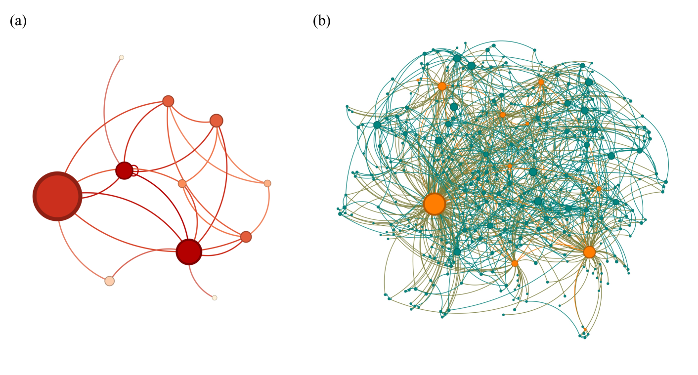
## Network Diagrams: Comparison of Sparse and Dense Network Topologies ### Overview The image presents two distinct network graphs, labeled (a) and (b). These diagrams visualize connectivity patterns, likely representing graph theory concepts or network analysis data. Diagram (a) depicts a small, sparse network with a monochromatic red-to-orange color scheme, while diagram (b) depicts a large, dense, complex network utilizing a bimodal color scheme of teal and orange. Both diagrams use node size to represent the degree of centrality or connectivity. ### Components/Axes * **Labels:** * **(a)**: Located at the top-left of the left diagram. * **(b)**: Located at the top-left of the right diagram. * **Nodes (Vertices):** Circular elements. The diameter of the circle corresponds to the node's degree centrality (the number of connections it possesses). * **Edges (Links):** Curved lines connecting the nodes. * **Color Coding:** * **Diagram (a):** A gradient from dark red (large, high-centrality nodes) to light orange/pink (small, low-centrality nodes). * **Diagram (b):** A bimodal palette. Orange nodes represent high-centrality hubs; teal nodes represent the majority of the network with lower centrality. ### Detailed Analysis #### Region (a): Sparse Network * **Structure:** This is a low-density network containing approximately 10–12 nodes. * **Connectivity:** The edges are clearly visible and distinct, allowing for the tracing of individual paths between nodes. * **Key Nodes:** * There is one dominant, large dark-red node positioned on the far left. * There is a secondary large dark-red node positioned in the lower-center. * The remaining nodes are significantly smaller and lighter in color, acting as peripheral points connected to the central hubs. * **Trend:** The network exhibits a "hub-and-spoke" tendency, where most connections radiate from or pass through the two largest nodes. #### Region (b): Dense Network * **Structure:** This is a high-density, large-scale network containing hundreds of nodes. It exhibits a "hairball" topology, where the density of edges makes individual path tracing impossible. * **Connectivity:** The network is highly interconnected. The edges form a dense web, suggesting a "small-world" network structure where the average path length between any two nodes is likely short. * **Key Nodes:** * There are two primary, large orange hubs: one located in the mid-left region and one in the lower-right region. * Several smaller orange nodes are scattered throughout the network, acting as secondary hubs. * The vast majority of the network consists of small teal nodes, which appear to be clustered around the orange hubs. * **Trend:** The distribution of node sizes suggests a scale-free network, where a few nodes (the orange hubs) possess a disproportionately high number of connections compared to the teal nodes. ### Key Observations * **Scale Contrast:** The image contrasts a manageable, observable network (a) with a complex, emergent system (b). * **Visual Complexity:** In (b), the density of the edges creates a visual "fog" in the center, indicating high levels of interaction or dependency between the nodes. * **Hub Dominance:** In both diagrams, the largest nodes are visually distinct (dark red in (a), orange in (b)), serving as the structural anchors for the rest of the network. ### Interpretation The data suggests a comparative study of network topology. * **Diagram (a)** likely represents a local community or a specific, small-scale interaction group where the relationships are explicit and easily mapped. The monochromatic color scheme suggests a single class of entities with varying degrees of influence. * **Diagram (b)** likely represents a global or systemic network (e.g., social media interactions, biological protein-protein interactions, or internet routing). The bimodal color scheme (teal vs. orange) implies a categorical distinction—perhaps distinguishing between "hubs" (orange) and "leaf nodes" or "peripheral nodes" (teal). The transition from (a) to (b) demonstrates how increasing the number of nodes and edges leads to emergent properties, where the network structure becomes defined by its hubs rather than individual connections. The "hairball" effect in (b) is a classic visualization challenge in network science, highlighting the difficulty of interpreting large-scale connectivity without algorithmic simplification.