## Chart: Logarithmic Plot of Calls vs. Clauses
### Overview
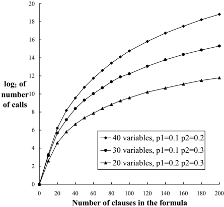
The image presents a chart illustrating the relationship between the number of clauses in a formula and the base-2 logarithm of the number of calls, for different numbers of variables and parameter settings. The chart uses three distinct lines to represent different configurations.
### Components/Axes
* **X-axis:** "Number of clauses in the formula", ranging from 0 to 200, with markers at 20, 40, 60, 80, 100, 120, 140, 160, 180, and 200.
* **Y-axis:** "log₂ of number of calls", ranging from 0 to 20, with markers at 2, 4, 6, 8, 10, 12, 14, 16, and 18.
* **Legend:** Located in the bottom-right corner, containing three entries:
* "40 variables, p1=0.1 p2=0.2" (represented by a black circle)
* "30 variables, p1=0.1 p2=0.3" (represented by a black circle)
* "20 variables, p1=0.2 p2=0.3" (represented by a black triangle)
### Detailed Analysis
The chart displays three curves, each representing a different set of parameters.
* **Line 1 (40 variables, p1=0.1 p2=0.2):** This line (black circles) exhibits a steadily increasing, concave-downward trend.
* At 20 clauses: log₂ of number of calls ≈ 2.1
* At 40 clauses: log₂ of number of calls ≈ 4.2
* At 60 clauses: log₂ of number of calls ≈ 6.1
* At 80 clauses: log₂ of number of calls ≈ 7.8
* At 100 clauses: log₂ of number of calls ≈ 9.4
* At 120 clauses: log₂ of number of calls ≈ 10.9
* At 140 clauses: log₂ of number of calls ≈ 12.4
* At 160 clauses: log₂ of number of calls ≈ 13.9
* At 180 clauses: log₂ of number of calls ≈ 15.4
* At 200 clauses: log₂ of number of calls ≈ 16.9
* **Line 2 (30 variables, p1=0.1 p2=0.3):** This line (black circles) also shows an increasing, concave-downward trend, but it consistently lies below Line 1.
* At 20 clauses: log₂ of number of calls ≈ 1.6
* At 40 clauses: log₂ of number of calls ≈ 3.5
* At 60 clauses: log₂ of number of calls ≈ 5.2
* At 80 clauses: log₂ of number of calls ≈ 6.8
* At 100 clauses: log₂ of number of calls ≈ 8.3
* At 120 clauses: log₂ of number of calls ≈ 9.7
* At 140 clauses: log₂ of number of calls ≈ 11.1
* At 160 clauses: log₂ of number of calls ≈ 12.5
* At 180 clauses: log₂ of number of calls ≈ 13.9
* At 200 clauses: log₂ of number of calls ≈ 15.2
* **Line 3 (20 variables, p1=0.2 p2=0.3):** This line (black triangles) exhibits the slowest growth, remaining below both Line 1 and Line 2.
* At 20 clauses: log₂ of number of calls ≈ 0.9
* At 40 clauses: log₂ of number of calls ≈ 2.5
* At 60 clauses: log₂ of number of calls ≈ 4.1
* At 80 clauses: log₂ of number of calls ≈ 5.6
* At 100 clauses: log₂ of number of calls ≈ 7.1
* At 120 clauses: log₂ of number of calls ≈ 8.5
* At 140 clauses: log₂ of number of calls ≈ 9.9
* At 160 clauses: log₂ of number of calls ≈ 11.3
* At 180 clauses: log₂ of number of calls ≈ 12.6
* At 200 clauses: log₂ of number of calls ≈ 13.9
### Key Observations
* The number of calls increases with the number of clauses for all parameter settings.
* Increasing the number of variables (from 20 to 40) leads to a higher number of calls for a given number of clauses.
* Increasing p2 (from 0.2 to 0.3) while keeping p1 constant, leads to a lower number of calls for a given number of clauses.
* The logarithmic scale on the Y-axis suggests that the relationship between the number of calls and the number of clauses is likely exponential.
### Interpretation
The chart demonstrates the computational cost associated with processing formulas with varying numbers of clauses and different parameter settings. The number of variables and the values of parameters p1 and p2 significantly influence the number of calls required. The logarithmic scale indicates that the computational cost grows exponentially with the number of clauses. This suggests that as the complexity of the formula (number of clauses) increases, the computational resources needed to process it grow rapidly. The differences between the lines highlight the importance of parameter tuning and variable management in optimizing performance. The data suggests that reducing the number of variables or adjusting the parameters can help mitigate the exponential growth in computational cost. The chart is likely illustrating the performance of a SAT solver or a similar constraint satisfaction algorithm.