## Line Chart: Epsilon Optimal vs. Alpha ### Overview The image contains a line chart showing the relationship between epsilon optimal (εopt) and alpha (α) for three different sigma values (σ1, σ2, σ3). The main chart displays a linear y-axis, while an inset chart in the top-right corner shows the same data with a logarithmic y-axis. The chart includes data points with error bars and fitted curves for each sigma value. ### Components/Axes * **Main Chart:** * **X-axis:** α (alpha), ranging from 0 to 4. * **Y-axis:** εopt (epsilon optimal), ranging from 0.0 to 1.2. * **Legend (bottom-right):** * Blue line: σ1 * Green line: σ2 * Red line: σ3 * **Inset Chart (top-right):** * **X-axis:** α (alpha), ranging from 1 to 4. * **Y-axis:** Logarithmic scale, ranging from 10^-3 to 10^-1. ### Detailed Analysis **Main Chart:** * **σ1 (Blue):** The blue line starts at approximately 1.0 at α = 0 and decreases rapidly until α ≈ 1.0. It then continues to decrease at a slower rate, reaching approximately 0.3 at α = 1.5, and then drops to approximately 0.1 at α = 3.0, remaining relatively constant thereafter. * α = 0: εopt ≈ 1.0 * α = 1.0: εopt ≈ 0.3 * α = 1.5: εopt ≈ 0.2 * α = 3.0: εopt ≈ 0.1 * α = 4.0: εopt ≈ 0.1 * **σ2 (Green):** The green line remains constant at approximately 1.0 from α = 0 to α ≈ 1.0. It then drops sharply to approximately 0.1 at α = 1.2, and continues to decrease to approximately 0.0 at α = 1.5, remaining relatively constant thereafter. * α = 0 to 1.0: εopt ≈ 1.0 * α = 1.2: εopt ≈ 0.1 * α = 1.5: εopt ≈ 0.0 * α = 4.0: εopt ≈ 0.0 * **σ3 (Red):** The red line starts at approximately 1.2 at α = 0 and decreases rapidly until α ≈ 1.5. It then continues to decrease at a slower rate, reaching approximately 0.4 at α = 2.0, and then drops to approximately 0.1 at α = 3.0, remaining relatively constant thereafter. * α = 0: εopt ≈ 1.2 * α = 1.5: εopt ≈ 0.4 * α = 2.0: εopt ≈ 0.3 * α = 3.0: εopt ≈ 0.1 * α = 4.0: εopt ≈ 0.1 **Inset Chart:** * **σ1 (Blue):** The blue line decreases from approximately 0.05 at α = 1.0 to approximately 0.001 at α = 4.0. * **σ2 (Green):** The green line decreases from approximately 0.08 at α = 1.0 to approximately 0.001 at α = 4.0. * **σ3 (Red):** The red line decreases from approximately 0.1 at α = 1.0 to approximately 0.002 at α = 4.0. ### Key Observations * All three sigma values show a decrease in εopt as α increases. * σ2 exhibits a sharp drop in εopt at α ≈ 1.0, while σ1 and σ3 show a more gradual decrease. * The inset chart provides a clearer view of the behavior of εopt at lower values, showing an exponential decay for all three sigma values. * The data points have error bars, indicating the uncertainty in the measurements. ### Interpretation The chart illustrates the relationship between epsilon optimal (εopt) and alpha (α) for different sigma values. The data suggests that as alpha increases, epsilon optimal decreases for all three sigma values. The sharp drop in εopt for σ2 indicates a critical point or threshold behavior, while the more gradual decrease for σ1 and σ3 suggests a more continuous relationship. The inset chart, with its logarithmic y-axis, highlights the exponential decay of εopt as alpha increases, particularly at lower values of εopt. The error bars on the data points indicate the variability or uncertainty in the measurements, which should be considered when interpreting the results. The different sigma values likely represent different experimental conditions or parameters, and the chart allows for a comparison of their effects on the relationship between epsilon optimal and alpha.

## Chart Type: Line Graph with Inset ### Overview This image is a technical scientific plot showing the relationship between a parameter $\alpha$ (on the x-axis) and an optimal error metric $\varepsilon^{\text{opt}}$ (on the y-axis). The graph displays three distinct data series, labeled $\sigma_1$, $\sigma_2$, and $\sigma_3$, each represented by a specific color (blue, green, and red, respectively). The plot includes both theoretical curves (solid and dashed lines) and experimental or simulated data points with error bars. An inset in the top-right corner provides a zoomed-in view of the lower error values on a logarithmic scale. ### Components/Axes * **Main Chart Region:** * **X-axis ($\alpha$):** Linear scale ranging from $0$ to $4$, with major tick marks every $1$ unit. * **Y-axis ($\varepsilon^{\text{opt}}$):** Linear scale ranging from $0.0$ to $1.2$, with major tick marks every $0.2$ units. * **Legend:** Located in the center-right area. * **Blue line:** $\sigma_1$ * **Green line:** $\sigma_2$ * **Red line:** $\sigma_3$ * **Inset Chart Region (Top-Right):** * **X-axis:** Linear scale from $1$ to $4$. * **Y-axis:** Logarithmic scale ranging from $10^{-3}$ to $10^{-1}$. * **Content:** Displays the tail-end decay of the three series on a log-linear scale. ### Detailed Analysis #### Component Isolation: Data Series Trends 1. **Series $\sigma_1$ (Blue):** * **Visual Trend:** The dashed line shows a continuous, smooth monotonic decrease. The solid line follows this decay until a critical point, where it drops abruptly to zero. * **Numerical Values:** * Starts at $\alpha = 0, \varepsilon^{\text{opt}} \approx 1.0$. * At $\alpha = 1.0, \varepsilon^{\text{opt}} \approx 0.35 \pm 0.02$. * At $\alpha = 2.0, \varepsilon^{\text{opt}} \approx 0.22 \pm 0.02$ (dashed line). * **Phase Transition:** At $\alpha \approx 3.05 \pm 0.05$, the solid blue line drops vertically from $\approx 0.15$ to $0$. * **Data Points:** Blue circles with error bars closely follow the dashed line. A few blue points (possibly diamonds) appear at lower values ($\varepsilon \approx 0.1$ to $0.05$) between $\alpha=2$ and $\alpha=3$. 2. **Series $\sigma_2$ (Green):** * **Visual Trend:** Stays perfectly flat at a high error value before undergoing a very sharp, discontinuous drop to a much lower error state. * **Numerical Values:** * Plateau at $\varepsilon^{\text{opt}} = 1.0$ for $\alpha \in [0, 1.1]$. * **Phase Transition:** At $\alpha \approx 1.12 \pm 0.03$, the solid line drops vertically from $1.0$ to $\approx 0.18$. * After the drop, it decays rapidly toward zero. At $\alpha = 2.0, \varepsilon^{\text{opt}} \approx 0.02 \pm 0.01$. * **Data Points:** Green circles follow the $1.0$ plateau and then track the lower branch after the transition. 3. **Series $\sigma_3$ (Red):** * **Visual Trend:** Similar to $\sigma_1$, it shows a smooth decay (dashed) and a discontinuous drop (solid) at an intermediate $\alpha$ value. * **Numerical Values:** * Starts at $\alpha = 0, \varepsilon^{\text{opt}} \approx 1.16 \pm 0.02$. * At $\alpha = 1.0, \varepsilon^{\text{opt}} \approx 0.50 \pm 0.03$. * **Phase Transition:** At $\alpha \approx 1.60 \pm 0.05$, the solid line drops vertically from $\approx 0.38$ to $\approx 0.10$. * **Data Points:** Red circles follow the upper dashed branch. Red diamonds follow the lower branch after the transition point. #### Inset Analysis The inset shows that for $\alpha > 2$, all three series exhibit an exponential decay (appearing as straight lines on the log-y plot). * **Relative Ordering:** In this high-$\alpha$ regime, $\sigma_2$ (green) has the lowest error, followed by $\sigma_3$ (red), and $\sigma_1$ (blue) has the highest error (among the non-zero branches). ### Key Observations * **Discontinuities:** All three series exhibit "jumps" or vertical drops in the solid lines, which are characteristic of first-order phase transitions. * **Metastability:** The presence of both dashed and solid lines suggests the existence of multiple solutions (e.g., global vs. local minima). The dashed lines likely represent metastable states that the system can stay in, while the solid lines represent the absolute optimal (global minimum) error. * **Initial Conditions:** $\sigma_3$ starts with a significantly higher initial error than $\sigma_1$ and $\sigma_2$. ### Interpretation This data likely represents a **Bayesian inference or machine learning task** (such as compressed sensing or a teacher-student neural network model) where $\alpha$ represents the measurement rate or sample complexity. 1. **Phase Transitions:** The sharp drops in $\varepsilon^{\text{opt}}$ indicate "learning transitions." Below a certain $\alpha$, the system is in a "poor" phase (high error). Once a critical amount of data ($\alpha_c$) is reached, the system can suddenly transition to a "good" phase (low error). 2. **The $\sigma_2$ Case:** The green series represents a scenario where no information is learned ($\varepsilon = 1.0$) until a threshold is met, after which learning is very efficient. This is typical of systems with a "hard" phase where local search algorithms might get stuck in the plateau. 3. **The $\sigma_1$ and $\sigma_3$ Cases:** These series show that some information is learned immediately as $\alpha$ increases, but a secondary transition still occurs where the error can be further minimized significantly. 4. **Asymptotic Behavior:** The inset confirms that once the system is in the "good" phase, the error decreases exponentially with more data, which is a standard result in many statistical learning problems. The different slopes in the inset suggest that the noise level or model parameters ($\sigma$) affect the rate of convergence.

## Chart: Optimal Error vs. Alpha ### Overview The image presents a line chart illustrating the relationship between the optimal error (εopt) and a parameter alpha (α). Three different curves, labeled σ1, σ2, and σ3, are plotted, each representing a different scenario or condition. The y-axis is on a linear scale, while the inset chart shows the same data on a logarithmic scale for the y-axis. Error bars are present for each data point, indicating the uncertainty in the measurements. ### Components/Axes * **X-axis:** Labeled "α" (alpha), ranging from approximately 0 to 4. * **Y-axis:** Labeled "εopt" (optimal error), ranging from approximately 0 to 1.2. The scale is linear. * **Inset Chart Y-axis:** Logarithmic scale, ranging from 10^-3 to 10^-1. * **Legend:** Located in the bottom-right corner, identifying the three curves: * σ1 (Blue solid line) * σ2 (Green solid line) * σ3 (Red dashed line) * **Error Bars:** Vertical lines indicating the uncertainty associated with each data point. ### Detailed Analysis **σ1 (Blue Line):** The blue line starts at approximately εopt = 0.8 at α = 0, and decreases rapidly to approximately εopt = 0.1 at α = 1. It then continues to decrease, leveling off around εopt = 0.02 at α = 3, and remains relatively constant until α = 4. * (0, 0.8) ± 0.1 * (1, 0.1) ± 0.02 * (2, 0.05) ± 0.01 * (3, 0.02) ± 0.005 * (4, 0.02) ± 0.005 **σ2 (Green Line):** The green line remains relatively constant at approximately εopt = 1.0 across the entire range of α, with some minor fluctuations indicated by the error bars. * (0, 1.0) ± 0.1 * (1, 1.0) ± 0.1 * (2, 1.0) ± 0.1 * (3, 1.0) ± 0.1 * (4, 1.0) ± 0.1 **σ3 (Red Line):** The red line starts at approximately εopt = 1.2 at α = 0 and decreases rapidly to approximately εopt = 0.4 at α = 1. It continues to decrease, reaching approximately εopt = 0.05 at α = 2, and then levels off around εopt = 0.02 at α = 3 and α = 4. * (0, 1.2) ± 0.1 * (1, 0.4) ± 0.05 * (2, 0.05) ± 0.01 * (3, 0.02) ± 0.005 * (4, 0.02) ± 0.005 ### Key Observations * The optimal error (εopt) decreases with increasing alpha (α) for both σ1 and σ3. * σ2 remains constant at a high error value, suggesting that the corresponding condition does not benefit from increasing alpha. * σ3 initially has a much higher optimal error than σ1, but both converge to similar low values at higher alpha values. * The inset chart provides a clearer view of the decreasing trends for all three curves, especially at lower error values. ### Interpretation The chart demonstrates how the optimal error changes as the parameter alpha is varied under three different conditions (σ1, σ2, and σ3). The decreasing trend of εopt with increasing α for σ1 and σ3 suggests that increasing alpha improves the performance or reduces the error in these scenarios. However, the constant high error for σ2 indicates that increasing alpha does not lead to any improvement in that specific condition. The convergence of σ1 and σ3 at higher alpha values suggests that the conditions represented by these two curves become more similar as alpha increases. The logarithmic scale in the inset chart highlights the rapid decrease in error at lower alpha values and the leveling off at higher alpha values. This could indicate diminishing returns from increasing alpha beyond a certain point. The error bars provide a measure of the uncertainty in the optimal error values, which is important for assessing the reliability of the results.

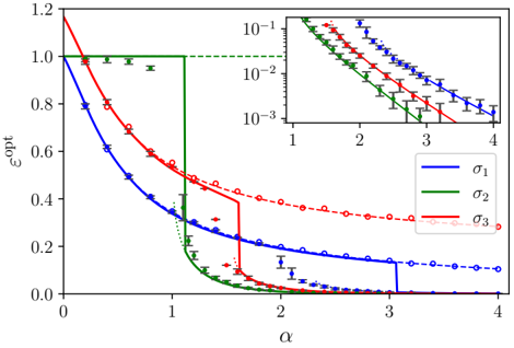
## Line Plot with Inset: Optimization Parameter (ε_opt) vs. α ### Overview The image is a scientific line plot displaying the relationship between a parameter `α` (x-axis) and an optimization parameter `ε_opt` (y-axis). It features three distinct data series labeled σ₁, σ₂, and σ₃, each plotted with both solid and dashed lines, along with error bars. A secondary inset plot in the top-right corner shows a subset of the data on a logarithmic y-axis scale. ### Components/Axes * **Main Plot Axes:** * **X-axis:** Label is `α`. Linear scale ranging from 0 to 4. Major tick marks at 0, 1, 2, 3, 4. * **Y-axis:** Label is `ε_opt`. Linear scale ranging from 0.0 to 1.2. Major tick marks at 0.0, 0.2, 0.4, 0.6, 0.8, 1.0, 1.2. * **Legend:** Located in the bottom-right quadrant of the main plot area. * `σ₁`: Blue line. * `σ₂`: Green line. * `σ₃`: Red line. * **Inset Plot:** Positioned in the top-right corner of the main plot. * **X-axis:** Linear scale, range approximately 1 to 4. Major tick marks at 1, 2, 3, 4. * **Y-axis:** Logarithmic scale. Labels at `10⁻³`, `10⁻²`, `10⁻¹`. * **Content:** Displays the same three data series (σ₁ blue, σ₂ green, σ₃ red) as lines with error bars, focusing on their behavior for `α` > 1 and `ε_opt` < 0.2. ### Detailed Analysis **Main Plot Data Series & Trends:** 1. **σ₁ (Blue):** * **Trend:** A smooth, monotonically decreasing curve. It starts at `ε_opt` ≈ 1.0 when `α`=0 and decays steadily. * **Key Points (Approximate):** * (`α`=0, `ε_opt`=1.0) * (`α`=1, `ε_opt`≈0.35) * (`α`=2, `ε_opt`≈0.15) * (`α`=3, `ε_opt`≈0.05) * (`α`=4, `ε_opt`≈0.02) * **Line Style:** Solid blue line connects data points. A dashed blue line continues the trend beyond `α`≈3.1. 2. **σ₂ (Green):** * **Trend:** Exhibits a sharp, discontinuous drop (phase transition). It remains constant at `ε_opt`=1.0 from `α`=0 until a critical point near `α`≈1.2, then plummets rapidly. * **Key Points & Features:** * Plateau: (`α`=0 to ~1.15, `ε_opt`=1.0). A horizontal dashed green line extends this plateau to `α`=4. * Critical Point: A vertical drop occurs at `α`≈1.2. * Post-drop: The curve decays quickly. At `α`=2, `ε_opt` is very close to 0. * **Line Style:** Solid green line for the plateau and initial drop. A dashed green line continues the low-value tail. 3. **σ₃ (Red):** * **Trend:** Shows a step-like decrease. It starts at `ε_opt`=1.2 when `α`=0, decays, then has a sharp vertical drop at `α`≈2.0. * **Key Points & Features:** * Start: (`α`=0, `ε_opt`=1.2). * Pre-step: Decays to (`α`≈1.9, `ε_opt`≈0.4). * Step: A vertical drop at `α`≈2.0. * Post-step: Continues decaying from a lower value. At `α`=3, `ε_opt`≈0.05. * **Line Style:** Solid red line for the initial decay and step. A dashed red line continues the trend beyond `α`≈2.0. **Inset Plot Analysis:** * The inset uses a logarithmic y-axis to emphasize the exponential decay behavior of the tails. * All three series (σ₁ blue, σ₂ green, σ₃ red) appear as roughly straight lines on this log-linear plot for `α` > 1.5, indicating exponential decay of the form `ε_opt ∝ exp(-kα)`. * The green line (σ₂) has the steepest slope (fastest decay), followed by red (σ₃), then blue (σ₁). ### Key Observations 1. **Distinct Behaviors:** The three σ parameters lead to fundamentally different optimization landscapes: smooth decay (σ₁), a sharp phase transition (σ₂), and a step-wise transition (σ₃). 2. **Critical Points:** σ₂ has a critical point at `α`≈1.2. σ₃ has a critical point at `α`≈2.0. σ₁ has no critical point. 3. **Asymptotic Behavior:** For large `α` (`α` > 3), all three `ε_opt` values converge towards zero, but at different rates, as confirmed by the inset. 4. **Initial Conditions:** At `α`=0, the starting `ε_opt` values differ: σ₃ starts highest (1.2), σ₁ and σ₂ start at 1.0. ### Interpretation This plot likely compares the performance or behavior of three different models, algorithms, or system configurations (parameterized by σ₁, σ₂, σ₃) as a control parameter `α` is varied. The `ε_opt` represents an error, cost, or inefficiency metric to be minimized. * **σ₁ (Blue)** represents a robust, stable system where performance degrades gracefully and predictably as `α` increases. * **σ₂ (Green)** represents a system with a **critical threshold** or **phase transition**. It maintains perfect performance (`ε_opt`=1.0) up to a tipping point (`α`≈1.2), after which it collapses rapidly. This is characteristic of systems with cooperative effects or bifurcations. * **σ₃ (Red)** represents a system with a **discrete mode switch**. It operates in one regime until `α`≈2.0, then abruptly switches to a more efficient, lower-error regime. This could indicate a change in strategy or the activation of a different mechanism. The inset confirms that in the high-`α` limit, all systems become exponentially efficient, but the transition path to that state is critically dependent on the underlying σ parameter. The choice between these behaviors (graceful degradation vs. threshold collapse vs. mode switch) would be a fundamental design decision depending on the application's tolerance for risk and need for stability.

## Line Graph: ε_opt vs α with Multiple Data Series ### Overview The image displays a line graph comparing the relationship between two variables: ε_opt (y-axis) and α (x-axis). Three distinct data series are plotted using different line styles and markers, with an inset graph showing a log-log scale version of the same data. The graph includes error bars for data points and a legend identifying the series. ### Components/Axes - **Primary Axes**: - **x-axis (α)**: Labeled "α", ranging from 0 to 4 in increments of 1. - **y-axis (ε_opt)**: Labeled "ε_opt", ranging from 0 to 1.2 in increments of 0.2. - **Inset Axes**: - **x-axis**: Labeled "α", ranging from 1 to 4 in increments of 1. - **y-axis**: Logarithmic scale labeled "10⁻¹", "10⁻²", "10⁻³". - **Legend**: Located in the bottom-right corner, associating: - **Blue solid line with circles**: σ₁ - **Green dashed line with squares**: σ₂ - **Red dotted line with triangles**: σ₃ ### Detailed Analysis 1. **σ₁ (Blue Solid Line)**: - Starts at ε_opt ≈ 1.2 when α = 0. - Drops sharply to ε_opt ≈ 0.4 at α = 1. - Plateaus near ε_opt ≈ 0.2 for α > 1. - Error bars are smallest at α = 0 and increase slightly at α = 1. 2. **σ₂ (Green Dashed Line)**: - Begins at ε_opt ≈ 0.8 when α = 0. - Dips to ε_opt ≈ 0.2 at α = 1. - Rises slightly to ε_opt ≈ 0.3 at α = 2, then declines again. - Error bars are largest at α = 1 and decrease afterward. 3. **σ₃ (Red Dotted Line)**: - Starts at ε_opt ≈ 1.0 when α = 0. - Decreases gradually to ε_opt ≈ 0.2 by α = 4. - Error bars remain consistent across α values. 4. **Inset Graph**: - All three series show exponential decay on the log-log scale. - σ₁ (blue) declines steepest, followed by σ₂ (green) and σ₃ (red). - Data points align closely with straight lines in the log-log plot, indicating power-law behavior. ### Key Observations - **σ₁** exhibits the most dramatic initial drop, suggesting a threshold effect at α = 1. - **σ₂** has a non-monotonic trend, with a local minimum at α = 1 and a secondary rise at α = 2. - **σ₃** shows the most gradual decline, maintaining higher ε_opt values longer than the other series. - The inset confirms that all series follow similar scaling laws, with σ₁ having the steepest decay rate. ### Interpretation The graph demonstrates how ε_opt varies with α under three distinct conditions (σ₁, σ₂, σ₃). The sharp drop in σ₁ at α = 1 implies a critical transition point, while σ₂'s dip and subsequent rise may indicate competing effects or non-linear interactions. The log-log inset reveals that all series share a common scaling behavior, with σ₁ being the most sensitive to changes in α. The error bars suggest increasing uncertainty in measurements as α increases, particularly for σ₂. This could reflect experimental limitations or inherent system variability at higher α values. The differing trends highlight the importance of σ parameters in determining ε_opt behavior, with potential applications in optimizing system performance or understanding phase transitions.