## Counterfactual Fairness Audit Density Plot
### Overview
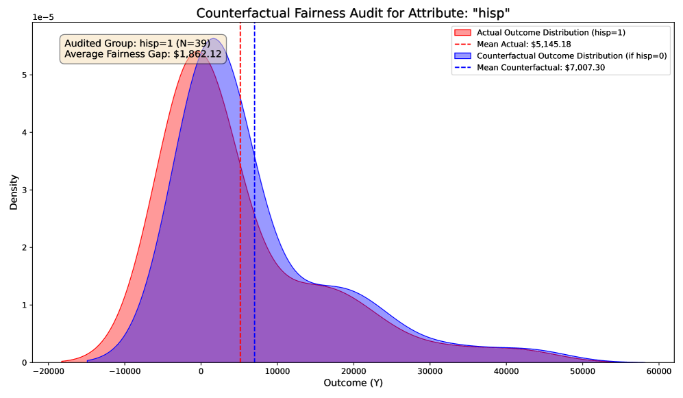
This image is a density plot visualizing a counterfactual fairness audit for the attribute "hisp" (likely an abbreviation for Hispanic). It compares the distribution of an outcome variable (Y) for an actual group (hisp=1) against a counterfactual distribution (if hisp=0). The chart includes summary statistics and a legend to differentiate the two distributions and their respective means.
### Components/Axes
* **Chart Title:** "Counterfactual Fairness Audit for Attribute: 'hisp'"
* **X-Axis:** Labeled "Outcome (Y)". The scale runs from approximately -20,000 to 60,000, with major tick marks at intervals of 10,000.
* **Y-Axis:** Labeled "Density". The scale runs from 0 to 5e-5 (0.00005), with major tick marks at intervals of 1e-5.
* **Legend (Top-Right Corner):**
* Red filled area: "Actual Outcome Distribution (hisp=1)"
* Red dashed vertical line: "Mean Actual: $5,145.18"
* Blue filled area: "Counterfactual Outcome Distribution (if hisp=0)"
* Blue dashed vertical line: "Mean Counterfactual: $7,007.30"
* **Annotation Box (Top-Left Corner):**
* "Audited Group: hisp=1 (N=39)"
* "Average Fairness Gap: $1,862.12"
### Detailed Analysis
* **Actual Outcome Distribution (hisp=1 - Red):**
* **Trend:** The distribution is right-skewed, with a sharp peak near an outcome value of 0 and a long tail extending towards higher positive values.
* **Key Points:** The density peaks at approximately 5.2e-5 on the y-axis. The mean is marked by a red dashed vertical line at $5,145.18 on the x-axis.
* **Counterfactual Outcome Distribution (if hisp=0 - Blue):**
* **Trend:** This distribution is also right-skewed but appears slightly shifted to the right compared to the red distribution. Its peak is slightly lower and broader.
* **Key Points:** The density peaks at approximately 5.0e-5 on the y-axis. The mean is marked by a blue dashed vertical line at $7,007.30 on the x-axis.
* **Comparison & Gap:**
* The two distributions overlap significantly, especially in the range from approximately -10,000 to 20,000.
* The blue (counterfactual) distribution has a visibly higher density for outcome values above approximately 5,000.
* The "Average Fairness Gap" is explicitly stated as $1,862.12, which is the difference between the two means ($7,007.30 - $5,145.18).
### Key Observations
1. **Right Skew:** Both outcome distributions are heavily right-skewed, indicating that most observations cluster around lower values, with a few high-value outliers pulling the mean to the right.
2. **Mean Displacement:** The counterfactual mean (if hisp=0) is higher than the actual mean (hisp=1) by $1,862.12. This is the central quantitative finding of the audit.
3. **Distribution Shape Difference:** While both are skewed, the counterfactual (blue) distribution appears to have a slightly heavier tail on the right side, suggesting a higher probability of very large outcomes in the counterfactual scenario.
4. **Small Sample Size:** The annotation notes the audited group (hisp=1) has a sample size of N=39, which is relatively small and should be considered when interpreting the robustness of the distributions.
### Interpretation
This chart demonstrates a **counterfactual fairness analysis**. It attempts to answer: "What would the outcome distribution look like for the same group of individuals if the sensitive attribute 'hisp' were changed from 1 to 0?"
* **What the Data Suggests:** The analysis suggests a potential disparity. For the same set of individuals (N=39), the model or system being audited produces a lower average outcome ($5,145.18) when the attribute is "hisp=1" compared to the hypothetical scenario where it is "hisp=0" ($7,007.30). The $1,862.12 gap quantifies this average disparity.
* **Relationship Between Elements:** The overlapping density plots show that the disparity is not uniform across all individuals; for many, the outcomes might be similar regardless of the attribute. However, the shift in the mean and the heavier right tail of the counterfactual distribution indicate that, on average and particularly for higher outcomes, the "hisp=0" scenario is associated with better results.
* **Notable Implications:** This type of audit is used to detect algorithmic bias. The finding implies that the attribute "hisp" is correlated with a lower outcome in the model's predictions or decisions, holding other factors constant (as implied by the counterfactual). The small sample size (N=39) is a limitation, suggesting this result may be specific to this subgroup and requires validation with larger data. The right-skewed nature of the outcomes (which could represent income, loan amounts, etc.) means the fairness gap has a more significant absolute impact on the higher end of the scale.