## Diagram: Comparison of Lean 4 Proofs - LLM vs. LLM + APOLLO
### Overview
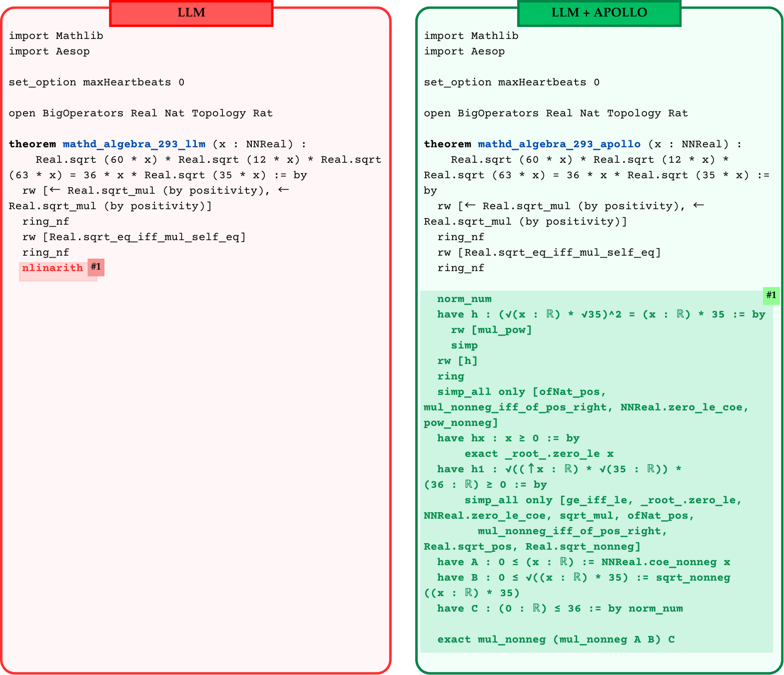
The image presents a side-by-side comparison of two formal mathematical proofs written in the Lean 4 theorem prover language. The graphic demonstrates how a standard Large Language Model (LLM) fails to complete a specific proof, whereas an augmented system ("LLM + APOLLO") successfully completes the same proof by replacing a failing high-level tactic with a detailed, step-by-step logical deduction.
### Components and Layout
The image is divided into two distinct vertical panels:
1. **Left Panel (LLM):**
* **Header:** A red rectangular tab at the top center containing the text "LLM" in black.
* **Border:** A thick red line with rounded corners enclosing the panel.
* **Background:** A very faint pink/red tint.
* **Content:** A block of Lean 4 code.
* **Annotation:** The final line of code (`nlinarith`) is highlighted with a red background, followed by a darker red tag reading `#1`.
2. **Right Panel (LLM + APOLLO):**
* **Header:** A green rectangular tab at the top center containing the text "LLM + APOLLO" in black.
* **Border:** A thick green line with rounded corners enclosing the panel.
* **Background:** A very faint green tint.
* **Content:** A block of Lean 4 code. The top half is nearly identical to the left panel.
* **Annotation:** The bottom half of the code is enclosed in a darker green highlighted box. In the top right corner of this highlighted box is a green tag reading `#1`.
### Content Details (Transcription)
Below is the exact transcription of the code presented in both panels.
#### Left Panel Transcription (LLM)
```lean
import Mathlib
import Aesop
set_option maxHeartbeats 0
open BigOperators Real Nat Topology Rat
theorem mathd_algebra_293_llm (x : NNReal) :
Real.sqrt (60 * x) * Real.sqrt (12 * x) * Real.sqrt (63 * x) = 36 * x * Real.sqrt (35 * x) := by
rw [← Real.sqrt_mul (by positivity), ← Real.sqrt_mul (by positivity)]
ring_nf
rw [Real.sqrt_eq_iff_mul_self_eq]
ring_nf
nlinarith #1
```
*(Note: The text `nlinarith #1` is highlighted in red in the original image).*
#### Right Panel Transcription (LLM + APOLLO)
```lean
import Mathlib
import Aesop
set_option maxHeartbeats 0
open BigOperators Real Nat Topology Rat
theorem mathd_algebra_293_apollo (x : NNReal) :
Real.sqrt (60 * x) * Real.sqrt (12 * x) * Real.sqrt (63 * x) = 36 * x * Real.sqrt (35 * x) := by
rw [← Real.sqrt_mul (by positivity), ← Real.sqrt_mul (by positivity)]
ring_nf
rw [Real.sqrt_eq_iff_mul_self_eq]
ring_nf
norm_num #1
have h : (√(x : ℝ) * √35)^2 = (x : ℝ) * 35 := by
rw [mul_pow]
simp
rw [h]
ring
simp_all only [ofNat_pos, mul_nonneg_iff_of_pos_right, NNReal.zero_le_coe, pow_nonneg]
have hx : x ≥ 0 := by
exact _root_.zero_le x
have h1 : √((↑x : ℝ) * √(35 : ℝ)) * (36 : ℝ) ≥ 0 := by
simp_all only [ge_iff_le, _root_.zero_le, NNReal.zero_le_coe, sqrt_mul, ofNat_pos, mul_nonneg_iff_of_pos_right, Real.sqrt_pos, Real.sqrt_nonneg]
have A : 0 ≤ (x : ℝ) := NNReal.coe_nonneg x
have B : 0 ≤ √((x : ℝ) * 35) := sqrt_nonneg ((x : ℝ) * 35)
have C : (0 : ℝ) ≤ 36 := by norm_num
exact mul_nonneg (mul_nonneg A B) C
```
*(Note: Everything from `norm_num` down to the end of the block is highlighted in green in the original image. The `#1` tag sits on the right margin aligned with `norm_num`).*
### Key Observations
* **Identical Setup:** Both scripts import the same libraries (`Mathlib`, `Aesop`), set the same options (`maxHeartbeats 0`), and open the same namespaces.
* **Theorem Statement:** The mathematical theorem being proved is identical: $\sqrt{60x} \cdot \sqrt{12x} \cdot \sqrt{63x} = 36x \cdot \sqrt{35x}$ where $x$ is a non-negative real number (`NNReal`). The only difference is the naming convention (`_llm` vs `_apollo`).
* **Initial Proof Steps:** The first four tactics applied in the `by` block are identical in both panels (`rw`, `ring_nf`, `rw`, `ring_nf`).
* **The Divergence (The `#1` Tag):**
* In the **LLM** panel, the model attempts to finish the proof using a single, powerful automated tactic: `nlinarith` (non-linear arithmetic). The red highlight indicates this tactic fails or times out.
* In the **LLM + APOLLO** panel, the failing `nlinarith` step is entirely replaced. The `#1` tag visually links the failure point on the left to the resolution block on the right.
* **The Resolution:** APOLLO replaces the single failing line with 22 lines of highly specific, step-by-step Lean 4 code. This new block manually handles type coercions (converting `NNReal` to `ℝ`), explicitly proves non-negativity (`have hx : x ≥ 0`, `have A : 0 ≤ (x : ℝ)`), and uses basic algebraic simplifications (`norm_num`, `simp`, `ring`) to satisfy the strict requirements of the theorem prover.
### Interpretation
This image serves as a technical demonstration of the limitations of standard LLMs in formal mathematics and the value of augmented systems (like "APOLLO").
**Reading between the lines:**
Standard LLMs possess strong "intuition" for mathematics. The LLM correctly recognized that the final step of this proof required resolving non-linear arithmetic, hence it guessed the `nlinarith` tactic. However, formal theorem provers like Lean 4 are pedantic; `nlinarith` often fails if the exact preconditions (like proving that variables inside square roots are strictly non-negative, or handling the invisible type coercions between non-negative reals and standard reals) are not explicitly laid out in the local context.
The "APOLLO" system appears to be an agentic framework or search mechanism that catches this failure. Instead of giving up, APOLLO takes the failing step (`#1`), analyzes the missing logical gaps, and generates the verbose, rigorous sub-proofs required to bridge the gap between the LLM's high-level intuition and Lean 4's strict type-checking engine. It proves that $x \ge 0$, that the square roots are valid, and that the multiplications hold, ultimately allowing the proof to compile successfully.