## [Code Comparison Diagram]: Lean 4 Theorem Proofs - LLM vs. LLM + APOLLO
### Overview
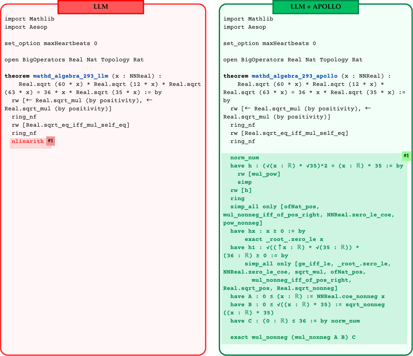
The image presents a side-by-side comparison of two Lean 4 code blocks, each containing a proof for the same mathematical theorem. The left block, outlined in red, is labeled "LLM". The right block, outlined in green, is labeled "LLM + APOLLO". The comparison visually highlights differences in the proof strategies and tactics employed by a standard Large Language Model (LLM) versus an LLM augmented with a system called APOLLO.
### Components/Axes
The image is divided into two primary, vertically oriented rectangular regions:
1. **Left Region (LLM):** Bordered in red. Contains a complete Lean 4 proof script.
2. **Right Region (LLM + APOLLO):** Bordered in green. Contains a complete Lean 4 proof script for the same theorem.
**Labels:**
* Top of Left Region: `LLM` (black text on a red background).
* Top of Right Region: `LLM + APOLLO` (black text on a green background).
**Embedded Annotations:**
* In the LLM proof, the tactic `nlinarith #1` is highlighted with a pink background.
* In the LLM + APOLLO proof, the annotation `#1` is highlighted with a green background at the end of the `norm_num` line.
### Detailed Analysis / Content Details
**Left Block (LLM) - Full Transcription:**
```lean
import Mathlib
import Aesop
set_option maxHeartbeats 0
open BigOperators Real Nat Topology Rat
theorem mathd_algebra_293_llm (x : NNReal) :
Real.sqrt (60 * x) * Real.sqrt (12 * x) * Real.sqrt (63 * x) = 36 * x * Real.sqrt (35 * x) := by
rw [← Real.sqrt_mul (by positivity), ← Real.sqrt_mul (by positivity)]
ring_nf
rw [Real.sqrt_eq_iff_mul_self_eq]
ring_nf
nlinarith #1
```
**Right Block (LLM + APOLLO) - Full Transcription:**
```lean
import Mathlib
import Aesop
set_option maxHeartbeats 0
open BigOperators Real Nat Topology Rat
theorem mathd_algebra_293_apollo (x : NNReal) :
Real.sqrt (60 * x) * Real.sqrt (12 * x) * Real.sqrt (63 * x) = 36 * x * Real.sqrt (35 * x) := by
rw [← Real.sqrt_mul (by positivity), ← Real.sqrt_mul (by positivity)]
ring_nf
rw [Real.sqrt_eq_iff_mul_self_eq]
ring_nf
norm_num #1
have h : (√(x : ℝ) * √35)^2 = (x : ℝ) * 35 := by
rw [mul_pow]
simp
rw [h]
ring
simp_all only [ofNat_pos, mul_nonneg_iff_of_pos_right, NNReal.zero_le_coe, pow_nonneg]
have hx : x ≥ 0 := by
exact _root_.zero_le x
have h1 : √((↑x : ℝ) * √(35 : ℝ)) * (36 : ℝ) ≥ 0 := by
simp_all only [ge_iff_le, _root_.zero_le, NNReal.zero_le_coe, sqrt_mul, ofNat_pos, mul_nonneg_iff_of_pos_right, Real.sqrt_pos, Real.sqrt_nonneg]
have A : 0 ≤ (x : ℝ) := NNReal.coe_nonneg x
have B : 0 ≤ √((x : ℝ) * 35) := sqrt_nonneg ((x : ℝ) * 35)
have C : (0 : ℝ) ≤ 36 := by norm_num
exact mul_nonneg (mul_nonneg A B) C
```
**Structural Comparison:**
* **Common Initial Steps:** Both proofs begin with identical setup (imports, options, open commands) and the same initial tactic sequence: two rewrites using `Real.sqrt_mul`, followed by `ring_nf`, a rewrite using `Real.sqrt_eq_iff_mul_self_eq`, and another `ring_nf`.
* **Divergence Point:** The proofs diverge after the second `ring_nf`.
* The **LLM** proof concludes with a single tactic: `nlinarith #1`.
* The **LLM + APOLLO** proof continues with a detailed, multi-step justification. It starts with `norm_num #1`, then establishes a helper lemma `h` about squaring a product of square roots, rewrites using it, applies `ring` and `simp_all`, and then explicitly constructs three hypotheses (`hx`, `h1`, `A`, `B`, `C`) to prove the non-negativity of the terms involved. The final step is `exact mul_nonneg (mul_nonneg A B) C`.
### Key Observations
1. **Proof Length and Explicitness:** The LLM + APOLLO proof is significantly longer and more verbose. It explicitly states and proves intermediate facts (like `h`, `hx`, `h1`, `A`, `B`, `C`) that the LLM proof likely leaves to the `nlinarith` tactic to infer.
2. **Tactic Choice:** The LLM relies on the powerful, automated `nlinarith` (nonlinear arithmetic) tactic to close the goal. The LLM + APOLLO version uses a combination of more basic tactics (`norm_num`, `ring`, `simp_all`) and explicit `have` statements to build the proof step-by-step.
3. **Visual Highlighting:** The pink highlight on `nlinarith #1` in the LLM block and the green highlight on `#1` in the LLM + APOLLO block draw attention to the critical, diverging steps in each proof.
4. **Theorem Naming:** The theorems are named `mathd_algebra_293_llm` and `mathd_algebra_293_apollo`, indicating they are two versions of the same problem (likely from a dataset like Mathlib's `mathd` series).
### Interpretation
This image is a technical comparison designed to showcase the effect of the "APOLLO" system on an LLM's code generation, specifically for formal theorem proving in Lean.
* **What it demonstrates:** It suggests that APOLLO guides the LLM to produce proofs that are more **explicit, structured, and possibly more reliable**. Instead of relying on a single, opaque automation tactic (`nlinarith`), the APOLLO-augmented model generates a proof that breaks down the reasoning into human-readable steps, explicitly verifying the non-negativity conditions required for the square root manipulations.
* **Relationship between elements:** The side-by-side layout forces a direct comparison. The identical initial steps establish a common baseline, making the divergence in the final proof strategy starkly clear. The color coding (red for baseline LLM, green for enhanced APOLLO) reinforces a "before/after" or "problem/solution" narrative.
* **Underlying message:** The detailed proof on the right is presented as superior—not necessarily because it's shorter (it's not), but because it is more transparent and constructs its argument from more fundamental principles. This aligns with goals in formal verification where proof clarity, maintainability, and independence from complex automation are highly valued. The image argues that APOLLO helps the LLM move from generating merely *correct* code to generating *well-structured, explanatory* code.