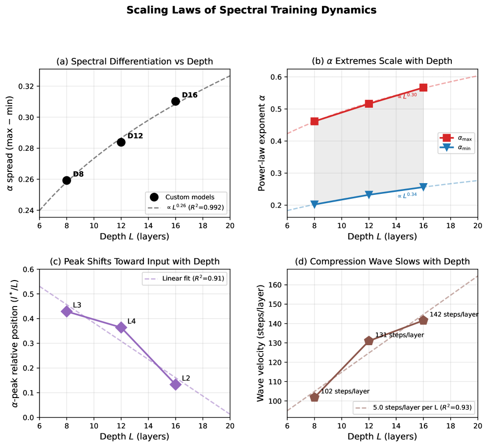
## Chart: Scaling Laws of Spectral Training Dynamics
### Overview
The image contains four subplots (a-d) illustrating scaling laws of spectral properties in neural networks as a function of network depth. Each subplot demonstrates a distinct spectral dynamic with depth, supported by mathematical fits and annotated data points.
---
### Components/Axes
#### Subplot (a): Spectral Differentiation vs Depth
- **X-axis**: Depth L (layers) [6–20]
- **Y-axis**: α spread (max − min) [0.24–0.32]
- **Legend**:
- Black circles: "Custom models"
- Dashed line: Linear fit (α ≈ L⁰.²⁶, R²=0.992)
- **Data points**:
- D8: α = 0.26
- D12: α = 0.28
- D16: α = 0.30
#### Subplot (b): α Extremes Scale with Depth
- **X-axis**: Depth L (layers) [6–20]
- **Y-axis**: Power-law exponent α [0.2–0.6]
- **Legend**:
- Red squares: α_max
- Blue triangles: α_min
- **Data points**:
- α_max:
- D8: 0.45
- D12: 0.5
- D16: 0.55
- D20: 0.6
- α_min:
- D8: 0.2
- D12: 0.23
- D16: 0.25
- **Fits**:
- α_max: α ≈ L⁰.³⁰ (R²=0.99)
- α_min: α ≈ L⁰.³⁴ (R²=0.98)
#### Subplot (c): Peak Shifts Toward Input with Depth
- **X-axis**: Depth L (layers) [6–20]
- **Y-axis**: α-peak relative position (I*/L) [0–0.6]
- **Legend**:
- Dashed line: Linear fit (R²=0.91)
- **Data points**:
- L2: 0.15
- L3: 0.35
- L4: 0.4
#### Subplot (d): Compression Wave Slows with Depth
- **X-axis**: Depth L (layers) [6–20]
- **Y-axis**: Wave velocity (steps/layer) [100–160]
- **Legend**:
- Dashed line: 5.0 steps/layer per L (R²=0.93)
- **Data points**:
- D8: 102 steps/layer
- D12: 131 steps/layer
- D16: 142 steps/layer
- D20: 160 steps/layer
---
### Detailed Analysis
#### Subplot (a)
- **Trend**: α spread increases monotonically with depth, following a power-law relationship (α ≈ L⁰.²⁶). The fit is exceptionally strong (R²=0.992).
- **Key values**:
- At L=8: α = 0.26
- At L=16: α = 0.30
#### Subplot (b)
- **Trend**:
- α_max increases sharply with depth (α ≈ L⁰.³⁰, R²=0.99).
- α_min increases more gradually (α ≈ L⁰.³⁴, R²=0.98).
- **Key values**:
- At L=8: α_max = 0.45, α_min = 0.2
- At L=16: α_max = 0.55, α_min = 0.25
#### Subplot (c)
- **Trend**: α-peak position decreases linearly with depth (R²=0.91), indicating peaks shift toward input as networks deepen.
- **Key values**:
- At L=2: 0.15
- At L=4: 0.35
- At L=3: 0.4 (peak at L=3)
#### Subplot (d)
- **Trend**: Wave velocity increases linearly with depth (5.0 steps/layer per L, R²=0.93).
- **Key values**:
- At L=8: 102 steps/layer
- At L=16: 142 steps/layer
- At L=20: 160 steps/layer
---
### Key Observations
1. **Consistent Scaling**: All subplots show strong power-law or linear relationships (R² > 0.91), suggesting predictable scaling laws.
2. **Divergent Dynamics**:
- Spectral differentiation (a) and α_max (b) increase with depth.
- α_min (b) and peak position (c) decrease with depth.
- Wave velocity (d) increases with depth.
3. **Depth Sensitivity**: Metrics like α spread (a) and wave velocity (d) show significant changes even between small depth increments (e.g., L=8 to L=12).
---
### Interpretation
The data demonstrates that spectral properties of neural networks scale systematically with depth, governed by power laws or linear relationships. These findings suggest:
- **Design Implications**: Predictable scaling allows for a priori estimation of spectral properties in deeper networks, aiding architectural choices.
- **Training Dynamics**: The compression wave slowing (d) may reflect increased computational complexity per layer in deeper networks.
- **Spectral Trade-offs**: The divergence between α_max and α_min (b) implies that deeper networks amplify certain spectral features while suppressing others, potentially affecting generalization or robustness.
The high R² values (0.91–0.992) validate the reliability of these scaling laws, making them actionable for both theoretical analysis and practical implementation.