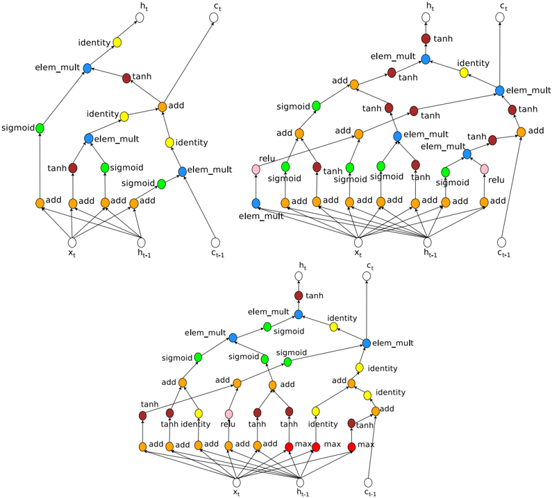
## Diagram: Recurrent Neural Network Cell Variations ### Overview The image presents three variations of a recurrent neural network (RNN) cell, likely Long Short-Term Memory (LSTM) or Gated Recurrent Unit (GRU) cells, visualized as computational graphs. Each cell takes inputs *x_t*, *h_t-1*, and *c_t-1* and produces outputs *h_t* and *c_t*. The diagrams illustrate the flow of data through different operations within each cell, such as sigmoid, tanh, element-wise multiplication (elem_mult), and addition (add). ### Components/Axes Each cell diagram contains the following components: * **Inputs:** * *x_t*: Input at time *t*. * *h_t-1*: Hidden state at time *t-1*. * *c_t-1*: Cell state at time *t-1*. * **Outputs:** * *h_t*: Hidden state at time *t*. * *c_t*: Cell state at time *t*. * **Operations:** * `sigmoid`: Sigmoid activation function. Represented by green nodes. * `tanh`: Hyperbolic tangent activation function. Represented by brown/dark red nodes. * `elem_mult`: Element-wise multiplication. Represented by blue nodes. * `add`: Addition. Represented by orange nodes. * `identity`: Identity function. Represented by yellow nodes. * `relu`: Rectified Linear Unit activation function. Represented by pink nodes. * `max`: Maximum function. Represented by red nodes. ### Detailed Analysis **Cell 1 (Top-Left)** * Input *x_t* is fed into three `add` operations. * Input *h_t-1* is fed into three `add` operations. * The outputs of these `add` operations are then passed through `tanh`, `sigmoid`, and `sigmoid` activations (green, brown, green). * The outputs of the `tanh` and `sigmoid` activations are combined using `elem_mult` (blue). * The output of the `elem_mult` is then passed through an `identity` function (yellow) to produce *h_t*. * Input *c_t-1* is passed through an `identity` function (yellow) and then combined with the output of another `elem_mult` (blue) via an `add` operation (orange). * The output of this `add` operation is passed through an `identity` function (yellow) to produce *c_t*. **Cell 2 (Top-Right)** * Input *x_t* is fed into four `add` operations. * Input *h_t-1* is fed into four `add` operations. * The outputs of these `add` operations are then passed through `tanh`, `sigmoid`, `sigmoid`, and `tanh` activations (brown, green, green, brown). * Input *c_t-1* is fed into four `add` operations. * The outputs of these `add` operations are then passed through `relu`, `sigmoid`, `sigmoid`, and `relu` activations (pink, green, green, pink). * The outputs of the `tanh` and `sigmoid` activations are combined using `elem_mult` (blue). * The output of the `elem_mult` is then passed through a `tanh` activation (brown) to produce *h_t*. * Input *c_t-1* is passed through an `identity` function (yellow) and then combined with the output of another `elem_mult` (blue) via an `add` operation (orange). * The output of this `add` operation is passed through an `elem_mult` function (blue) to produce *c_t*. **Cell 3 (Bottom)** * Input *x_t* is fed into four `add` operations. * Input *h_t-1* is fed into three `max` operations (red). * Input *c_t-1* is fed into three `max` operations (red). * The outputs of these `add` operations are then passed through `tanh`, `identity`, `relu`, and `tanh` activations (brown, yellow, pink, brown). * The outputs of the `tanh` and `sigmoid` activations are combined using `elem_mult` (blue). * The output of the `elem_mult` is then passed through a `tanh` activation (brown) to produce *h_t*. * Input *c_t-1* is passed through an `identity` function (yellow) and then combined with the output of another `elem_mult` (blue) via an `add` operation (orange). * The output of this `add` operation is passed through an `identity` function (yellow) to produce *c_t*. ### Key Observations * Each cell processes inputs *x_t*, *h_t-1*, and *c_t-1* differently, using various combinations of activation functions and operations. * The `elem_mult` operation is a key component in combining the outputs of different activation functions. * The `add` operation is used to combine the inputs with the outputs of previous operations. * The `identity` function is used to pass the cell state *c_t-1* to the next time step. * The variations in the cells likely represent different architectures or design choices for RNNs. ### Interpretation The diagrams illustrate the computational flow within three different RNN cell architectures. These cells likely represent variations of LSTM or GRU cells, which are designed to address the vanishing gradient problem in traditional RNNs. The different combinations of activation functions, element-wise multiplications, and additions allow each cell to learn different patterns in the input data. The presence of cell state *c_t* allows the network to store and propagate information across time steps, enabling it to capture long-range dependencies in sequential data. The variations in the cells likely reflect different trade-offs between computational complexity and performance on specific tasks.

\n ## Diagram: LSTM Cell Structure ### Overview The image depicts three variations of the Long Short-Term Memory (LSTM) cell structure, a type of recurrent neural network architecture. Each cell diagram illustrates the flow of information through various gates and operations. The diagrams are arranged in a 3x1 grid, with the top diagram being the most simplified, the middle diagram being more complex, and the bottom diagram being the most complex. ### Components/Axes The diagrams utilize the following components: * **Nodes:** Representing data values (x_t, h_t, c_t, n_t-1, c_t-1). * **Operations:** Represented by labeled circles or boxes (add, sigmoid, tanh, relu, max, elem\_mult, identity). * **Connections:** Lines with arrows indicating the direction of data flow. * **Input:** x_t * **Previous Hidden State:** h_t-1 * **Previous Cell State:** c_t-1 * **Current Hidden State:** h_t * **Current Cell State:** c_t ### Detailed Analysis or Content Details **Top LSTM Cell:** * **Inputs:** x_t, h_t-1, c_t-1 * **Operations:** * Multiple "add" operations combining inputs. * "sigmoid" activations. * "tanh" activations. * "elem\_mult" (element-wise multiplication). * "identity" connections (direct pass-through). * **Outputs:** h_t, c_t * **Flow:** x_t and h_t-1 are combined through multiple "add" operations and passed through "sigmoid" and "tanh" activations. These outputs are then combined with c_t-1 via "elem\_mult" and "add" operations to produce c_t. h_t is derived from a similar pathway. **Middle LSTM Cell:** * **Inputs:** x_t, h_t-1, c_t-1 * **Operations:** * Multiple "add" operations. * "sigmoid" activations. * "tanh" activations. * "relu" activations. * "elem\_mult" (element-wise multiplication). * "identity" connections. * **Outputs:** h_t, c_t * **Flow:** Similar to the top cell, but with the addition of "relu" activations and a more complex network of "add" and "elem\_mult" operations. **Bottom LSTM Cell:** * **Inputs:** x_t, h_t-1, c_t-1 * **Operations:** * Multiple "add" operations. * "sigmoid" activations. * "tanh" activations. * "relu" activations. * "max" operations. * "elem\_mult" (element-wise multiplication). * "identity" connections. * **Outputs:** h_t, c_t * **Flow:** The most complex of the three, featuring "max" operations alongside the other operations. The flow is highly interconnected, with multiple pathways for data to travel through. ### Key Observations * The complexity of the LSTM cell increases from top to bottom. * All three cells share the core components of "add", "sigmoid", "tanh", "elem\_mult", and "identity" operations. * The addition of "relu" and "max" operations in the lower cells suggests more sophisticated gate mechanisms. * The diagrams illustrate the core principle of LSTM cells: maintaining and updating a cell state (c_t) while selectively allowing information to flow through gates controlled by sigmoid activations. ### Interpretation The diagrams demonstrate the evolution of the LSTM cell architecture. The top diagram represents a simplified version, while the middle and bottom diagrams showcase increasingly complex implementations designed to improve the cell's ability to learn long-term dependencies in sequential data. The addition of "relu" and "max" operations likely contributes to more nuanced gate control and improved performance. The diagrams highlight the core concept of LSTM cells: the use of gates to regulate the flow of information, enabling the network to selectively remember or forget information over time. The consistent presence of x_t, h_t-1, and c_t-1 as inputs and h_t and c_t as outputs across all three diagrams emphasizes the fundamental input-output relationship of the LSTM cell. The diagrams are not providing specific numerical data, but rather a visual representation of the computational structure of the LSTM cell. They are conceptual diagrams, not charts or graphs.

## Neural Network Architecture Diagrams: Recurrent Cell Variants ### Overview The image displays three distinct computational graphs representing different recurrent neural network cell architectures. Each diagram illustrates the flow of data from inputs (\(x_t\), \(h_{t-1}\), \(c_{t-1}\)) to outputs (\(h_t\), \(c_t\)) through a series of mathematical operations. The nodes are color-coded by operation type, and the connections show the data dependencies. The diagrams are arranged with two at the top (left and right) and one centered below them. ### Components/Axes * **Inputs (Bottom of each graph):** Three white circular nodes labeled: * \(x_t\) (current input) * \(h_{t-1}\) (previous hidden state) * \(c_{t-1}\) (previous cell state) * **Outputs (Top of each graph):** Two white circular nodes labeled: * \(h_t\) (current hidden state) * \(c_t\) (current cell state) * **Operation Nodes (Color-coded):** * **Orange:** `add` (addition) * **Blue:** `elem_mult` (element-wise multiplication) * **Green:** `sigmoid` (sigmoid activation) * **Dark Red/Brown:** `tanh` (hyperbolic tangent activation) * **Yellow:** `identity` (pass-through) * **Pink:** `relu` (Rectified Linear Unit activation) - *Present only in the top-right and bottom diagrams.* * **Red:** `max` (maximum operation) - *Present only in the bottom diagram.* * **Connections:** Directed lines (edges) showing the flow of data from one operation to the next. ### Detailed Analysis #### **Diagram 1 (Top-Left)** * **Structure:** Relatively simple, with a clear separation between pathways leading to \(h_t\) and \(c_t\). * **Flow to \(h_t\):** The path involves a combination of `sigmoid`, `tanh`, `elem_mult`, and `add` operations. The final output \(h_t\) is derived from an `elem_mult` node combining a `tanh`-activated signal and a `sigmoid`-gated signal. * **Flow to \(c_t\):** The cell state update involves an `add` operation combining the previous cell state \(c_{t-1}\) (via an `identity` node) with a new candidate value. This candidate is generated through a series of `sigmoid`, `tanh`, and `elem_mult` operations. * **Key Operations:** Uses `sigmoid` gates, `tanh` for candidate values, and `elem_mult` for gating. No `relu` or `max` operations are present. #### **Diagram 2 (Top-Right)** * **Structure:** More complex and interconnected than the first diagram. Features a denser network of operations in the lower half. * **Flow to \(h_t\):** The path to the hidden state is intricate, involving multiple `add`, `tanh`, and `elem_mult` nodes. It incorporates a `relu` activation (pink node) in one of the lower pathways. * **Flow to \(c_t\):** The cell state update is also more complex, with multiple parallel pathways feeding into the final `add` node that updates \(c_{t-1}\) to \(c_t\). It includes an `identity` connection from \(c_{t-1}\). * **Key Operations:** Introduces a `relu` activation. The architecture has a higher degree of connectivity and more `add` operations in the initial processing layers compared to Diagram 1. #### **Diagram 3 (Bottom)** * **Structure:** Distinct from the top two, characterized by a prominent row of `add` and `max` operations at the very bottom, just above the inputs. * **Flow to \(h_t\):** The hidden state is produced via a path involving `sigmoid`, `elem_mult`, and `tanh` operations. It features a `relu` activation (pink node) in one branch. * **Flow to \(c_t\):** The cell state update mechanism is unique. It uses an `add` node that combines: 1. The previous cell state \(c_{t-1}\) via an `identity` path. 2. A signal that has passed through a `max` operation (red node). * **Key Operations:** The most notable feature is the use of `max` operations (red nodes) in the initial processing layer, which is not present in the other two diagrams. This suggests a different form of non-linear combination or pooling of the input and recurrent signals. ### Key Observations 1. **Common Framework:** All three diagrams share the same fundamental input/output structure (\(x_t, h_{t-1}, c_{t-1} \rightarrow h_t, c_t\)) and use a similar set of core operations (`add`, `elem_mult`, `sigmoid`, `tanh`, `identity`). 2. **Increasing Complexity:** There is a visual progression in complexity from the top-left (simplest) to the top-right and then to the bottom diagram. 3. **Architectural Variations:** * **Activation Functions:** Diagram 1 uses only `sigmoid` and `tanh`. Diagrams 2 and 3 introduce `relu`. * **Novel Operation:** Diagram 3 uniquely incorporates `max` operations, suggesting a different gating or combination mechanism. * **Connectivity:** The density of connections and the number of parallel pathways increase from Diagram 1 to Diagrams 2 and 3. 4. **Spatial Layout:** The legend (color-to-operation mapping) is implicit but consistent across all three diagrams. The inputs are always at the bottom, outputs at the top, with data flowing upward. ### Interpretation These diagrams are technical schematics for **Recurrent Neural Network (RNN) cells**, specifically variants of Long Short-Term Memory (LSTM) or Gated Recurrent Unit (GRU) architectures. They visually encode the mathematical equations that define how the cell's hidden state and cell state are updated at each time step. * **What they demonstrate:** The image compares three different design choices for constructing a recurrent cell. The variations lie in the specific arrangement of operations and the inclusion of different activation functions (`relu`) or combination functions (`max`). * **Relationship between elements:** The `sigmoid` nodes likely represent **gates** (controlling information flow), the `tanh` nodes represent **candidate value generation**, and the `elem_mult` nodes implement the **gating mechanism** itself. The `add` nodes perform state updates. The `max` operation in the third diagram could represent a form of **dynamic routing** or **selective activation** of pathways. * **Significance:** This is a **Peircean** representation of architectural hypotheses. Each diagram is a "sign" (the drawing) representing an "object" (a specific RNN cell formula) to an "interpretant" (a researcher). The differences suggest an exploration of how to improve gradient flow, model capacity, or computational efficiency. The inclusion of `relu` and `max` points towards attempts to mitigate the vanishing gradient problem or to introduce more complex, non-linear interactions within the cell. The bottom diagram's `max` operation is particularly notable as it deviates from the standard additive/multiplicative paradigm of LSTMs, potentially offering a different inductive bias for learning temporal dependencies.

## Diagram: Neural Network Computational Graph ### Overview The image depicts three interconnected computational graphs representing neural network operations, likely from a recurrent architecture (e.g., LSTM/GRU). Nodes represent mathematical operations/activations, while edges indicate data flow. Three diagrams are stacked vertically, showing progressive complexity with shared components. ### Components/Axes - **Nodes**: - **Red**: `tanh` (hyperbolic tangent activation) - **Blue**: `elem_mult` (element-wise multiplication) - **Green**: `sigmoid` (sigmoid activation) - **Orange**: `add` (element-wise addition) - **Yellow**: `identity` (no-op operation) - **Pink**: `relu` (rectified linear unit) - **Labels**: - Input: `x_t` (current time step input) - Hidden states: `h_t` (current), `h_t-1` (previous) - Cell states: `c_t` (current), `c_t-1` (previous) - **Flow Direction**: Left-to-right (typical for sequential processing). ### Detailed Analysis 1. **Top Diagram**: - **Structure**: - `x_t` → `tanh` (red) → `elem_mult` (blue) → `add` (orange) → `h_t` (output). - `h_t-1` and `c_t-1` feed into `elem_mult` and `add` operations. - **Key Connections**: - `tanh` output is element-wise multiplied with `h_t-1` (blue node). - Result added to `c_t-1` (orange `add` node) to produce `h_t`. 2. **Middle Diagram**: - **Structure**: - Expands on top diagram with additional `sigmoid` (green) and `identity` (yellow) nodes. - `sigmoid` gates modulate `elem_mult` operations. - **Key Connections**: - `sigmoid` outputs control element-wise multiplications (e.g., `sigmoid` → `elem_mult` → `add`). - `identity` nodes preserve values for skip connections. 3. **Bottom Diagram**: - **Structure**: - Most complex, with `max` operations (red) and `relu` (pink). - Introduces parallel paths for gradient computation. - **Key Connections**: - `max` operations aggregate gradients across multiple paths. - `relu` applied to intermediate states for non-linearity. ### Key Observations - **Skip Connections**: `identity` nodes enable residual connections, preserving gradients during backpropagation. - **Temporal Dependency**: `h_t-1` and `c_t-1` propagate information across time steps. - **Color Consistency**: Node colors align with their labels (e.g., all `tanh` nodes are red). - **Gradient Flow**: `max` operations in the bottom diagram suggest attention mechanisms or gradient clipping. ### Interpretation This diagram illustrates the forward and backward passes of a recurrent neural network, likely an LSTM cell. The `tanh` and `sigmoid` gates regulate information flow, while `elem_mult` and `add` combine hidden/cell states. The `max` and `relu` operations in the bottom diagram hint at advanced variants (e.g., attention or gradient regulation). The graphs emphasize modularity, with reusable components (e.g., `elem_mult` blocks) and efficient computation through element-wise operations. The absence of explicit numerical values suggests this is a conceptual representation rather than empirical data.