TECHNICAL ASSET FINGERPRINT
c98ed201f7e42fd939017cce
Click to view fullscreen
Press ESC or click to close
FOUND IN PAPERS
EXPERT: healer-alpha-free VERSION 1
RUNTIME: free/openrouter/healer-alpha
INTEL_VERIFIED
\n
## Multi-Panel Chart: Multi-Agent Hybrid Pursuit-Evasion Game Analysis
### Overview
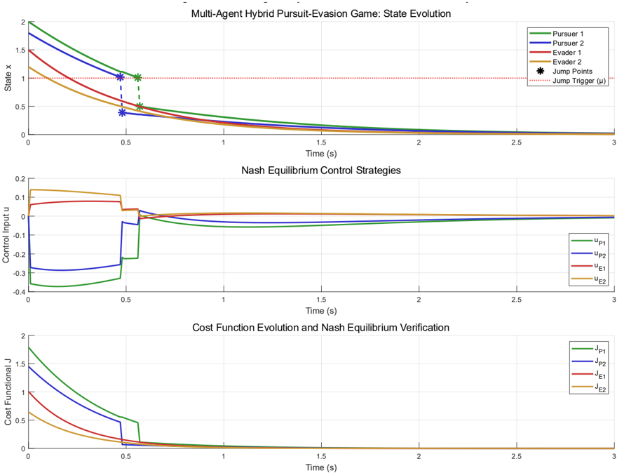
The image displays three vertically stacked time-series plots analyzing a "Multi-Agent Hybrid Pursuit-Evasion Game." The plots share a common x-axis representing "Time (s)" from 0 to 3 seconds. The top plot shows the state evolution of four agents, the middle plot shows their Nash Equilibrium control strategies, and the bottom plot shows the evolution of their cost functions. The system exhibits a hybrid dynamic, with discontinuous jumps in state and control occurring at specific times.
### Components/Axes
* **Overall Title:** "Multi-Agent Hybrid Pursuit-Evasion Game: State Evolution"
* **Common X-Axis (All Plots):** Label: "Time (s)". Scale: Linear, from 0 to 3 with major ticks at 0, 0.5, 1, 1.5, 2, 2.5, 3.
* **Top Plot:**
* **Title:** "Multi-Agent Hybrid Pursuit-Evasion Game: State Evolution"
* **Y-Axis:** Label: "State x". Scale: Linear, from 0 to 2 with major ticks at 0, 0.5, 1, 1.5, 2.
* **Legend (Top-Right):**
* Green Line: "Pursuer 1"
* Blue Line: "Pursuer 2"
* Red Line: "Evader 1"
* Orange Line: "Evader 2"
* Black Asterisk (*): "Jump Points"
* Red Dotted Line: "Jump Trigger (μ)"
* **Middle Plot:**
* **Title:** "Nash Equilibrium Control Strategies"
* **Y-Axis:** Label: "Control Input u". Scale: Linear, from -0.4 to 0.2 with major ticks at -0.4, -0.3, -0.2, -0.1, 0, 0.1, 0.2.
* **Legend (Top-Right):**
* Green Line: "u_P1" (Control for Pursuer 1)
* Blue Line: "u_P2" (Control for Pursuer 2)
* Red Line: "u_E1" (Control for Evader 1)
* Orange Line: "u_E2" (Control for Evader 2)
* **Bottom Plot:**
* **Title:** "Cost Function Evolution and Nash Equilibrium Verification"
* **Y-Axis:** Label: "Cost Functional J". Scale: Linear, from 0 to 2 with major ticks at 0, 0.5, 1, 1.5, 2.
* **Legend (Top-Right):**
* Green Line: "J_P1" (Cost for Pursuer 1)
* Blue Line: "J_P2" (Cost for Pursuer 2)
* Red Line: "J_E1" (Cost for Evader 1)
* Orange Line: "J_E2" (Cost for Evader 2)
### Detailed Analysis
**1. State Evolution (Top Plot):**
* **Trend:** All four agents' state variables (`x`) decrease over time, converging towards zero. The lines are smooth curves except for discontinuities.
* **Initial States (t=0s):** Pursuer 1 (Green) ≈ 2.0, Pursuer 2 (Blue) ≈ 1.8, Evader 1 (Red) ≈ 1.5, Evader 2 (Orange) ≈ 1.2.
* **Jump Trigger:** A horizontal red dotted line at `x = 1.0` is labeled "Jump Trigger (μ)".
* **Jump Points:** Black asterisks mark discontinuities where the state trajectories jump.
* **First Jump (t ≈ 0.45s):** Pursuer 2 (Blue) jumps down from ~0.9 to ~0.4. Evader 1 (Red) jumps down from ~0.8 to ~0.5.
* **Second Jump (t ≈ 0.55s):** Pursuer 1 (Green) jumps down from ~1.1 to ~0.5. Evader 2 (Orange) jumps down from ~0.7 to ~0.5.
* **Post-Jump Behavior:** After t ≈ 0.6s, all states continue a smooth, asymptotic decay towards zero. By t=3s, all states are very close to 0.
**2. Nash Equilibrium Control Strategies (Middle Plot):**
* **Trend:** Control inputs (`u`) show piecewise continuous segments with sharp discontinuities at the jump times (t ≈ 0.45s and 0.55s). After the jumps, controls converge towards zero.
* **Initial Controls (t=0s):** Pursuer 1 (Green) ≈ -0.38, Pursuer 2 (Blue) ≈ -0.28, Evader 1 (Red) ≈ 0.08, Evader 2 (Orange) ≈ 0.14.
* **Control at First Jump (t ≈ 0.45s):** Controls for Pursuer 2 (Blue) and Evader 1 (Red) exhibit sharp changes. Pursuer 2's control jumps from ~-0.28 to ~-0.05. Evader 1's control jumps from ~0.08 to ~0.03.
* **Control at Second Jump (t ≈ 0.55s):** Controls for Pursuer 1 (Green) and Evader 2 (Orange) exhibit sharp changes. Pursuer 1's control jumps from ~-0.32 to ~-0.22. Evader 2's control jumps from ~0.1 to ~0.05.
* **Steady-State:** After t ≈ 1s, all control inputs are very small in magnitude and slowly approach zero.
**3. Cost Function Evolution (Bottom Plot):**
* **Trend:** All cost functionals (`J`) decrease monotonically over time, converging to zero. They exhibit discontinuities at the same jump times as the state and control plots.
* **Initial Costs (t=0s):** Pursuer 1 (Green) ≈ 1.8, Pursuer 2 (Blue) ≈ 1.5, Evader 1 (Red) ≈ 1.0, Evader 2 (Orange) ≈ 0.6.
* **Cost at Jumps:** The cost curves for each agent show a sharp, vertical drop at their respective jump times (t ≈ 0.45s for P2/E1, t ≈ 0.55s for P1/E2).
* **Final Costs:** By t=3s, all cost functionals have converged to a value very close to 0.
### Key Observations
1. **Hybrid System Dynamics:** The system is clearly hybrid, with continuous evolution punctuated by discrete jumps triggered when a state crosses the threshold `μ = 1.0`.
2. **Synchronized Agent Pairs:** The jumps occur in pairs: Pursuer 2 and Evader 1 jump together at ~0.45s; Pursuer 1 and Evader 2 jump together at ~0.55s. This suggests a coupling or interaction rule between specific pursuer-evader pairs.
3. **Convergence to Equilibrium:** All states, controls, and costs converge towards zero as time progresses, indicating the system reaches a stable equilibrium (likely a capture or meeting point).
4. **Cost Hierarchy:** The initial and transient costs maintain a consistent order: J_P1 > J_P2 > J_E1 > J_E2. This suggests Pursuer 1 has the highest initial cost or performance objective, while Evader 2 has the lowest.
5. **Control Effort:** Pursuers (negative control) exert effort to decrease the state, while Evaders (positive control) exert effort to increase it, consistent with a pursuit-evasion game. The magnitude of control effort diminishes after the jumps.
### Interpretation
This data visualizes the solution to a multi-agent differential game with hybrid dynamics. The "Nash Equilibrium" label indicates the plotted strategies are such that no agent can unilaterally improve its outcome.
* **Game Dynamics:** The pursuers aim to minimize the state `x` (likely representing distance or a capture condition), while the evaders aim to maximize it. The control inputs reflect this antagonistic relationship.
* **Role of the Hybrid Jump:** The jump at `x = μ` acts as a reset or capture mechanism. When an agent's state reaches this threshold, it undergoes a discrete transition, significantly reducing its state value and cost. This could model events like a sensor detection, a capture attempt, or a change in engagement rules.
* **Strategic Coupling:** The paired jumps imply the game's rules or cost functions create strategic dependencies between specific pursuer-evader teams (P1-E2 and P2-E1). The actions or state of one directly trigger a reset for its paired opponent.
* **Efficiency of the Equilibrium:** The smooth, convergent trajectories post-jump and the monotonic decrease in cost functionals suggest the Nash equilibrium strategies are effective and stable, leading the system to a terminal state (capture/evasion endgame) in finite time. The diminishing control effort indicates the agents' strategies become less aggressive as the game resolves.
In summary, the charts depict a well-defined hybrid pursuit-evasion game where agents follow optimal strategies that lead to a predictable, convergent outcome, with discrete jumps playing a critical role in resetting the system's state and accelerating convergence.
DECODING INTELLIGENCE...