\n
## Chart: Cumulative Probability vs. Peak Size for Different k and W Values
### Overview
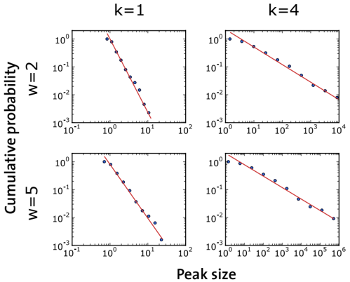
The image presents four separate log-log plots, each displaying the cumulative probability of peak size. The plots are arranged in a 2x2 grid, with varying values of 'k' (1 and 4) and 'W' (2 and 5). Each plot shows a scatter of blue data points fitted with a red line. The x-axis represents "Peak size" and the y-axis represents "Cumulative probability". Both axes are on a logarithmic scale.
### Components/Axes
* **X-axis Label:** "Peak size" (logarithmic scale)
* **Y-axis Label:** "Cumulative probability" (logarithmic scale)
* **Titles:** Each subplot is labeled with 'k' and 'W' values:
* Top-left: k=1, W=2
* Top-right: k=4, W=2
* Bottom-left: k=1, W=5
* Bottom-right: k=4, W=5
* **Data Points:** Blue circles representing observed data.
* **Fitted Lines:** Red lines representing the fitted cumulative distribution.
* **Axis Scales:** Both axes range from approximately 10^-1 to 10^6 on the logarithmic scale.
### Detailed Analysis
Each subplot will be analyzed individually.
**1. k=1, W=2 (Top-left)**
* **Trend:** The data points show a clear downward trend, indicating that as peak size increases, cumulative probability decreases. The line is approximately linear on the log-log scale.
* **Data Points (approximate):**
* Peak size ≈ 10^-1, Cumulative probability ≈ 10^1
* Peak size ≈ 10^0, Cumulative probability ≈ 10^0.5 (approximately 3)
* Peak size ≈ 10^1, Cumulative probability ≈ 10^-0.5 (approximately 0.3)
* Peak size ≈ 10^2, Cumulative probability ≈ 10^-1.5 (approximately 0.03)
**2. k=4, W=2 (Top-right)**
* **Trend:** Similar downward trend as the first plot, but the decrease is less steep. The line is also approximately linear on the log-log scale.
* **Data Points (approximate):**
* Peak size ≈ 10^-1, Cumulative probability ≈ 10^1
* Peak size ≈ 10^0, Cumulative probability ≈ 10^0.7 (approximately 5)
* Peak size ≈ 10^1, Cumulative probability ≈ 10^-0.3 (approximately 0.5)
* Peak size ≈ 10^4, Cumulative probability ≈ 10^-1.5 (approximately 0.03)
**3. k=1, W=5 (Bottom-left)**
* **Trend:** Downward trend, similar to k=1, W=2, but the data points are more scattered. The line is approximately linear on the log-log scale.
* **Data Points (approximate):**
* Peak size ≈ 10^-1, Cumulative probability ≈ 10^1
* Peak size ≈ 10^0, Cumulative probability ≈ 10^0.5 (approximately 3)
* Peak size ≈ 10^1, Cumulative probability ≈ 10^-0.5 (approximately 0.3)
* Peak size ≈ 10^2, Cumulative probability ≈ 10^-1.5 (approximately 0.03)
**4. k=4, W=5 (Bottom-right)**
* **Trend:** Downward trend, similar to k=4, W=2, but the decrease is less steep. The line is also approximately linear on the log-log scale.
* **Data Points (approximate):**
* Peak size ≈ 10^-1, Cumulative probability ≈ 10^1
* Peak size ≈ 10^0, Cumulative probability ≈ 10^0.7 (approximately 5)
* Peak size ≈ 10^1, Cumulative probability ≈ 10^-0.3 (approximately 0.5)
* Peak size ≈ 10^5, Cumulative probability ≈ 10^-1.5 (approximately 0.03)
### Key Observations
* All four plots exhibit a power-law relationship between peak size and cumulative probability, as evidenced by the approximately linear trend on the log-log scale.
* Increasing 'k' (from 1 to 4) results in a less steep slope, indicating a slower decrease in cumulative probability with increasing peak size.
* Increasing 'W' (from 2 to 5) appears to have a minor effect on the slope, but the data is more scattered for W=5.
* The data points are relatively well-fitted by the red lines, suggesting a good model fit.
### Interpretation
The plots demonstrate the cumulative distribution of peak sizes for different parameter settings (k and W). The power-law behavior suggests that large peaks are relatively rare, while small peaks are more common. The parameter 'k' appears to control the rate at which the probability of observing a peak decreases with increasing peak size. A higher 'k' value implies a slower decay, meaning larger peaks are more likely to occur. The parameter 'W' may influence the overall distribution shape, but its effect is less pronounced and the data is more variable. These plots could be used to characterize the distribution of events in a system where peak sizes are important, such as earthquake magnitudes, financial market fluctuations, or network traffic bursts. The differences in the slopes for different 'k' values suggest that the underlying process generating these peaks is sensitive to the 'k' parameter. The fact that the lines are approximately linear on a log-log scale indicates that the distribution follows a power law, which is often observed in complex systems.