## Log-Log Scatter Plots: Cumulative Probability vs. Peak Size
### Overview
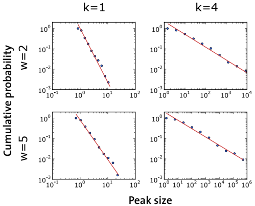
The image displays a 2x2 grid of four scatter plots. Each plot shows the relationship between "Peak size" (x-axis) and "Cumulative probability" (y-axis) on logarithmic scales. The plots are differentiated by two parameters: `k` (columns: 1 and 4) and `w` (rows: 2 and 5). Each plot contains blue data points and a fitted red trend line, suggesting a power-law or similar heavy-tailed distribution.
### Components/Axes
* **Grid Structure:** A 2x2 matrix of subplots.
* **Top-Left:** Title `k=1`, `w=2`
* **Top-Right:** Title `k=4`, `w=2`
* **Bottom-Left:** Title `k=1`, `w=5`
* **Bottom-Right:** Title `k=4`, `w=5`
* **X-Axis (All Plots):** Label: `Peak size`. Scale: Logarithmic (base 10).
* For `k=1` plots (left column): Range approximately from `10^-1` to `10^2`.
* For `k=4` plots (right column): Range approximately from `10^0` to `10^4` (top-right) and `10^0` to `10^6` (bottom-right).
* **Y-Axis (All Plots):** Label: `Cumulative probability`. Scale: Logarithmic (base 10). Range approximately from `10^-3` to `10^0` (i.e., 0.001 to 1).
* **Data Series:** Each plot contains a series of blue circular data points.
* **Trend Line:** Each plot contains a solid red line representing a linear fit to the data on the log-log scale.
### Detailed Analysis
**Plot 1 (Top-Left: k=1, w=2):**
* **Trend:** The blue data points follow a steep, downward-sloping linear trend on the log-log plot.
* **Data Points (Approximate):** The series starts near `(Peak size ≈ 10^0, Cumulative probability ≈ 10^0)` and ends near `(Peak size ≈ 10^1, Cumulative probability ≈ 10^-3)`.
* **Slope:** The red trend line has a steep negative slope, approximately -3 (calculated as (log10(10^-3) - log10(10^0)) / (log10(10^1) - log10(10^0)) = (-3 - 0)/(1 - 0) = -3).
**Plot 2 (Top-Right: k=4, w=2):**
* **Trend:** The blue data points follow a less steep, downward-sloping linear trend compared to the k=1 case.
* **Data Points (Approximate):** The series starts near `(Peak size ≈ 10^0, Cumulative probability ≈ 10^0)` and ends near `(Peak size ≈ 10^4, Cumulative probability ≈ 10^-2)`.
* **Slope:** The red trend line has a moderate negative slope, approximately -0.5 (estimated as (log10(10^-2) - log10(10^0)) / (log10(10^4) - log10(10^0)) = (-2 - 0)/(4 - 0) = -0.5).
**Plot 3 (Bottom-Left: k=1, w=5):**
* **Trend:** The blue data points follow a steep, downward-sloping linear trend, very similar to the k=1, w=2 plot.
* **Data Points (Approximate):** The series starts near `(Peak size ≈ 10^0, Cumulative probability ≈ 10^0)` and ends near `(Peak size ≈ 10^1.5, Cumulative probability ≈ 10^-3)`.
* **Slope:** The red trend line has a steep negative slope, approximately -2 (estimated as (log10(10^-3) - log10(10^0)) / (log10(10^1.5) - log10(10^0)) ≈ (-3 - 0)/(1.5 - 0) = -2).
**Plot 4 (Bottom-Right: k=4, w=5):**
* **Trend:** The blue data points follow a shallow, downward-sloping linear trend, spanning the widest range on the x-axis.
* **Data Points (Approximate):** The series starts near `(Peak size ≈ 10^0, Cumulative probability ≈ 10^0)` and ends near `(Peak size ≈ 10^6, Cumulative probability ≈ 10^-2)`.
* **Slope:** The red trend line has a very shallow negative slope, approximately -0.33 (estimated as (log10(10^-2) - log10(10^0)) / (log10(10^6) - log10(10^0)) = (-2 - 0)/(6 - 0) ≈ -0.33).
### Key Observations
1. **Parameter `k` Dominates Slope:** The most significant visual difference is between the left column (`k=1`) and the right column (`k=4`). The `k=1` plots show a much steeper decline in cumulative probability with increasing peak size compared to the `k=4` plots.
2. **Parameter `w` Affects Range:** For a fixed `k`, increasing `w` from 2 to 5 extends the range of the x-axis (`Peak size`) over which the data is plotted, particularly noticeable for `k=4` (from ~10^4 to ~10^6).
3. **Power-Law Behavior:** The linear relationship on the log-log plots strongly suggests that the cumulative probability `P(X ≥ x)` follows a power-law distribution of the form `P(X ≥ x) ∝ x^(-α)`, where the negative slope of the red line corresponds to the exponent `-α`.
4. **Consistent Starting Point:** All four distributions appear to start at a cumulative probability of 1 (10^0) for the smallest peak sizes (~10^0), which is typical for a complementary cumulative distribution function (CCDF).
### Interpretation
These plots likely analyze the statistical distribution of "peak sizes" from a system or process governed by parameters `k` and `w`. The power-law behavior indicates a heavy-tailed distribution, meaning very large peaks, while rare, are more probable than they would be in a normal (Gaussian) distribution.
* **The parameter `k` appears to control the "heaviness" of the tail.** A lower `k` (k=1) results in a steeper slope (larger exponent α), meaning the probability of observing very large peaks decays rapidly. A higher `k` (k=4) results in a shallower slope (smaller exponent α), indicating a "heavier" tail where extreme events are relatively more likely.
* **The parameter `w` seems to influence the scale or observation window** of the process, as it extends the maximum observed peak size without drastically changing the fundamental slope (for a given `k`).
**In a practical context,** this could model phenomena like earthquake magnitudes, city sizes, or failure sizes in complex systems. The analysis shows that tuning `k` dramatically changes the risk profile (likelihood of extreme events), while `w` might relate to the system's size or duration of observation. The clear separation of trends by `k` suggests it is the primary control parameter for the underlying generative mechanism.