## Scatter Plots: Cumulative Probability vs. Peak Size (Log-Log Scale)
### Overview
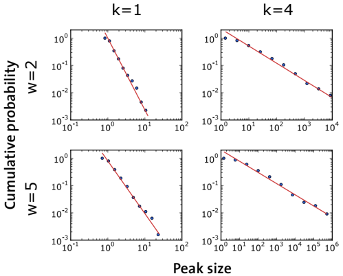
The image contains four scatter plots arranged in a 2x2 grid, each depicting the relationship between **peak size** (x-axis, log scale) and **cumulative probability** (y-axis, log scale). The plots are labeled with parameters:
- **Top row**: `k=1` (left) and `k=4` (right)
- **Bottom row**: `w=2` (left) and `w=5` (right)
Each plot includes blue data points and a red trend line, suggesting a power-law relationship between peak size and cumulative probability.
---
### Components/Axes
- **X-axis (Peak size)**: Logarithmic scale from $10^{-1}$ to $10^6$.
- **Y-axis (Cumulative probability)**: Logarithmic scale from $10^{-3}$ to $10^0$.
- **Legend**: No explicit legend, but the red line represents a fitted trend.
- **Titles**:
- Top-left: `k=1`
- Top-right: `k=4`
- Bottom-left: `w=2`
- Bottom-right: `w=5`
---
### Detailed Analysis
#### Top-left (`k=1`, `w=2`):
- **Data points**: Blue dots follow a steep downward trend.
- **Trend line**: Red line slopes sharply, indicating a strong inverse relationship.
- **Key values**:
- At peak size $10^0$, cumulative probability ≈ $10^{-1}$.
- At peak size $10^2$, cumulative probability ≈ $10^{-2}$.
#### Top-right (`k=4`, `w=2`):
- **Data points**: Blue dots show a less steep decline compared to `k=1`.
- **Trend line**: Red line has a shallower slope, suggesting a weaker inverse relationship.
- **Key values**:
- At peak size $10^0$, cumulative probability ≈ $10^{-1}$.
- At peak size $10^4$, cumulative probability ≈ $10^{-3}$.
#### Bottom-left (`k=1`, `w=5`):
- **Data points**: Blue dots exhibit a moderate decline.
- **Trend line**: Red line slopes between the `k=1` and `k=4` plots.
- **Key values**:
- At peak size $10^0$, cumulative probability ≈ $10^{-1}$.
- At peak size $10^2$, cumulative probability ≈ $10^{-2}$.
#### Bottom-right (`k=4`, `w=5`):
- **Data points**: Blue dots show the least steep decline.
- **Trend line**: Red line has the shallowest slope, indicating the weakest inverse relationship.
- **Key values**:
- At peak size $10^0$, cumulative probability ≈ $10^{-1}$.
- At peak size $10^6$, cumulative probability ≈ $10^{-3}$.
---
### Key Observations
1. **Inverse relationship**: All plots show a clear negative correlation between peak size and cumulative probability.
2. **Parameter dependence**:
- Higher `k` values (e.g., `k=4`) reduce the steepness of the trend, implying larger peak sizes are more probable.
- Higher `w` values (e.g., `w=5`) also reduce the steepness, suggesting broader distributions of peak sizes.
3. **Consistency**: The red trend lines align with the blue data points, confirming the power-law behavior.
---
### Interpretation
The data demonstrates that **cumulative probability decreases exponentially with peak size**, but the rate of decrease depends on parameters `k` and `w`:
- **Larger `k`**: Reduces the sensitivity of cumulative probability to peak size, favoring larger peaks.
- **Larger `w`**: Similarly broadens the distribution, making extreme peak sizes less probable.
- **Power-law scaling**: The log-log plots confirm a power-law relationship, where cumulative probability $P \propto \text{peak size}^{-\alpha}$, with $\alpha$ decreasing as `k` or `w` increases.
This suggests that the system’s behavior is governed by a balance between `k` (possibly a scaling factor) and `w` (possibly a width or dispersion parameter), with both parameters modulating the distribution of peak sizes.