## Line Chart: Learning Rate Schedule
### Overview
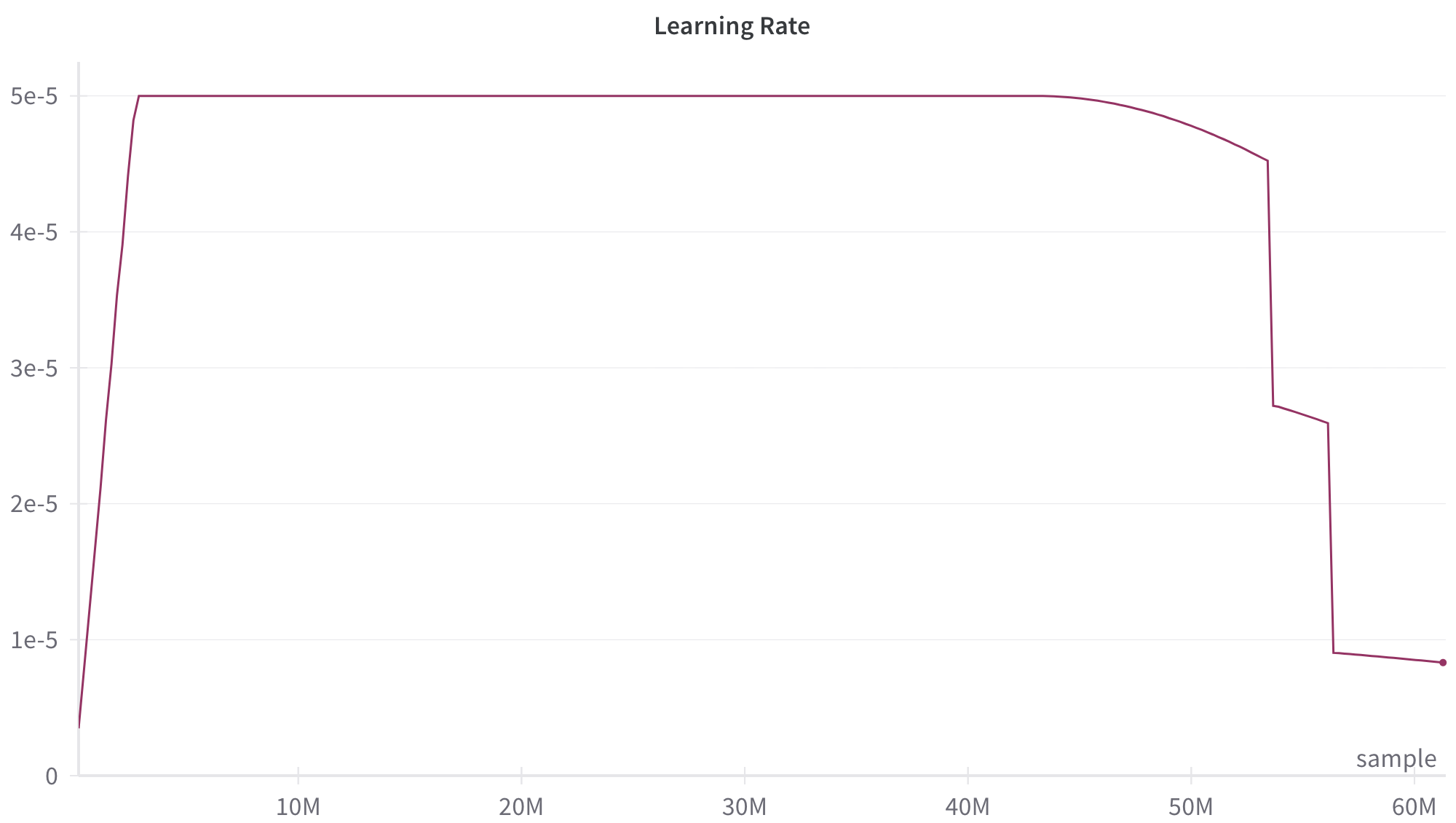
This image is a line chart displaying the trajectory of a "Learning Rate" over a specific number of training "samples." The chart illustrates a complex learning rate schedule characterized by an initial warm-up, a prolonged constant phase, a gradual decay, and two distinct, sharp step-downs near the end of the training run.
*Language Declaration:* All text in this image is in English.
### Components/Axes
**Header Region:**
* **Title:** "Learning Rate" (Positioned top-center).
**Main Chart Region:**
* **Data Series:** A single continuous line plotted in a dark maroon/purple color.
* **Gridlines:** Faint, light gray horizontal gridlines correspond to the major Y-axis markers. There are faint vertical tick marks on the X-axis, but no vertical gridlines extending through the chart.
**Y-Axis (Left):**
* **Label:** None explicitly stated, but represents the learning rate value.
* **Scale:** Linear, utilizing scientific notation.
* **Markers (Bottom to Top):**
* 0
* 1e-5
* 2e-5
* 3e-5
* 4e-5
* 5e-5
**X-Axis (Bottom):**
* **Label:** "sample" (Positioned at the bottom-right, just above the axis line).
* **Scale:** Linear, representing millions of samples (denoted by 'M').
* **Markers (Left to Right):**
* (Origin is 0, though not explicitly marked with a 0 on the x-axis line itself, it aligns with the y-axis 0).
* 10M
* 20M
* 30M
* 40M
* 50M
* 60M
### Detailed Analysis
The dark maroon line exhibits several distinct visual trends, which can be broken down into sequential phases:
1. **Initial Warm-up (Steep Upward Slope):**
* *Trend:* The line starts near the bottom-left origin and slopes upward almost vertically.
* *Data Points:* It begins at approximately `x = 0`, `y = 0.3e-5`. It rises sharply to reach the maximum value of `y = 5e-5` at approximately `x = 2M` samples.
2. **Constant Phase (Flat Horizontal Line):**
* *Trend:* The line becomes perfectly flat, moving horizontally to the right.
* *Data Points:* The learning rate is held constant at `5e-5` from approximately `x = 2M` to `x = 44M` samples.
3. **Initial Decay (Smooth Downward Curve):**
* *Trend:* The line begins to curve downward smoothly, resembling the beginning of a cosine decay.
* *Data Points:* Starting at `x = 44M`, the value gradually drops from `5e-5` to approximately `4.5e-5` at `x = 53.5M`.
4. **First Step-Down (Sharp Vertical Drop):**
* *Trend:* The line drops almost vertically.
* *Data Points:* At approximately `x = 53.5M`, the value plummets from `~4.5e-5` down to `~2.7e-5`.
5. **Intermediate Decay (Slight Downward Slope):**
* *Trend:* The line resumes a very gradual downward slope.
* *Data Points:* From `x = 53.5M` to `x = 56M`, the value decreases slightly from `~2.7e-5` to `~2.6e-5`.
6. **Second Step-Down (Sharp Vertical Drop):**
* *Trend:* The line experiences a second near-vertical drop.
* *Data Points:* At approximately `x = 56M`, the value falls sharply from `~2.6e-5` down to `~0.9e-5`.
7. **Final Decay (Slight Downward Slope to Terminus):**
* *Trend:* The line continues with a very slight downward slope until it ends at a distinct circular marker (dot).
* *Data Points:* From `x = 56M` to just past the 60M mark (approximately `x = 61M`), the value decays from `~0.9e-5` to a final plotted point at `~0.8e-5`.
### Key Observations
* **Dominant Phase:** The vast majority of the training (roughly 70% of the total samples) occurs at the peak, constant learning rate of `5e-5`.
* **Anomalous Drops:** The smooth decay is interrupted by two very sudden, discrete drops in the learning rate at ~53.5M and ~56M samples. This is not typical of a standard continuous decay schedule (like pure linear or cosine).
* **Explicit Terminus:** The graph ends with a specific dot marker, indicating the exact end of the training run or schedule.
### Interpretation
This chart represents a highly customized learning rate schedule used in training a machine learning model (likely a deep neural network, given the scale of 60 million samples).
* **The Warm-up:** The initial steep climb is a standard "warm-up" phase. This is used to prevent the model from diverging early in training when gradients can be unstable, allowing the network to safely reach the optimal base learning rate.
* **The Plateau:** The long flat period at `5e-5` is where the bulk of the generalized learning occurs. The model is taking large, consistent steps to find the general area of the global minima in the loss landscape.
* **The Complex Decay:** The latter portion of the graph (from 44M onwards) is highly specific. It begins as a smooth decay (likely to help the model settle into a local minima), but the sudden step-downs suggest a hybrid approach. This could represent a "Step Decay" schedule overlaid on a smooth curve, or it could indicate manual interventions/restarts by the researcher. Often, these sharp drops are triggered when validation loss plateaus; dropping the learning rate drastically allows the model to fine-tune and escape a saddle point or settle deeper into a narrow minima.
* **Overall Strategy:** The schedule prioritizes rapid, broad learning for the first 75% of the run, followed by aggressive, multi-stage fine-tuning in the final 25% to squeeze out maximum performance.