## Diagram: Commutative Diagram of K-Theory ### Overview The image is a commutative diagram illustrating relationships between different K-theory groups. It shows how various maps (denoted by arrows) connect these groups, with labels indicating the specific transformations or operations being applied. ### Components/Axes The diagram consists of the following components: * **Nodes:** These represent K-theory groups, labeled as: * `K^T(Z(f^A + g^A))` (top-left) * `K^T(Z(f^A))` (top-right) * `K^T(X^A, f^A + g^A)` (center-left) * `K^T(X^A, f^A)` (center-right) * `K^T(X, f + g)` (middle-left) * `K^T(X, f)` (middle-right) * `K^T(Z(f + g))` (bottom-left) * `K^T(Z(f))` (bottom-right) * **Arrows:** These represent maps between the K-theory groups, labeled as: * `sp^A` (top horizontal arrow) * `can` (diagonal arrows from top corners to center nodes) * `Stab_e^s` (vertical arrows from center nodes to middle nodes, and from top-right to bottom-right, and top-left to bottom-left) * `sp` (horizontal arrow from middle-left to middle-right, and bottom horizontal arrow) * `can` (diagonal arrows from middle nodes to bottom corners) ### Detailed Analysis or Content Details The diagram shows the following relationships: 1. `K^T(Z(f^A + g^A))` maps to `K^T(Z(f^A))` via `sp^A`. 2. `K^T(Z(f^A + g^A))` maps to `K^T(X^A, f^A + g^A)` via `can`. 3. `K^T(Z(f^A))` maps to `K^T(X^A, f^A)` via `can`. 4. `K^T(X^A, f^A + g^A)` maps to `K^T(X^A, f^A)` via `sp^A`. 5. `K^T(X^A, f^A + g^A)` maps to `K^T(X, f + g)` via `Stab_e^s`. 6. `K^T(X^A, f^A)` maps to `K^T(X, f)` via `Stab_e^s`. 7. `K^T(Z(f^A + g^A))` maps to `K^T(Z(f + g))` via `Stab_e^s`. 8. `K^T(Z(f^A))` maps to `K^T(Z(f))` via `Stab_e^s`. 9. `K^T(X, f + g)` maps to `K^T(X, f)` via `sp`. 10. `K^T(X, f + g)` maps to `K^T(Z(f + g))` via `can`. 11. `K^T(X, f)` maps to `K^T(Z(f))` via `can`. 12. `K^T(Z(f + g))` maps to `K^T(Z(f))` via `sp`. ### Key Observations * The diagram is structured in a square-like fashion, with two rows and two columns of K-theory groups. * The maps `sp^A` and `sp` appear to represent some form of specialization or projection. * The maps `can` likely represent canonical maps or inclusions. * The maps `Stab_e^s` likely represent stabilization maps. ### Interpretation The diagram illustrates the relationships between different K-theory groups under various transformations. The commutativity of the diagram implies that the composition of maps along different paths between the same starting and ending points yields the same result. This suggests that the diagram represents a well-defined structure in K-theory, where the different maps are compatible with each other. The specific meaning of the maps `sp^A`, `sp`, `can`, and `Stab_e^s` would require further context within the field of K-theory. The diagram likely demonstrates how different constructions in K-theory are related and how they interact with each other.

## Commutative Diagram: Algebraic K-Theory/Stabilization Maps ### Overview The image displays a commutative diagram from advanced mathematics, likely within the fields of algebraic topology, homotopy theory, or algebraic K-theory. It illustrates the relationships and compatibility between several functors or constructions (denoted by `K^T`) applied to different objects (`Z`, `X`) and functions (`f`, `g`), under the operations of stabilization (`Stab^A_e`), specialisation (`sp`, `sp^A`), and canonical maps (`can`). The diagram is structured as a 3x3 grid of nodes connected by horizontal, vertical, and diagonal arrows. ### Components/Axes (Nodes and Arrows) **Nodes (9 total, arranged in a grid):** * **Top Row (Left to Right):** 1. `K^T(Z(f^A + g^A))` 2. (Arrow target, no node) 3. `K^T(Z(f^A))` * **Middle Row (Left to Right):** 1. `K^T(X^A, f^A + g^A)` 2. (Arrow target, no node) 3. `K^T(X^A, f^A)` * **Bottom Row (Left to Right):** 1. `K^T(Z(f + g))` 2. `K^T(X, f + g)` 3. `K^T(X, f)` 4. `K^T(Z(f))` **Arrows and Labels:** * **Horizontal Arrows:** * Top: `K^T(Z(f^A + g^A))` → `K^T(Z(f^A))` labeled `sp^A`. * Middle: `K^T(X^A, f^A + g^A)` → `K^T(X^A, f^A)` labeled `sp^A`. * Middle-Lower: `K^T(X, f + g)` → `K^T(X, f)` labeled `sp`. * Bottom: `K^T(Z(f + g))` → `K^T(Z(f))` labeled `sp`. * **Vertical Arrows:** * Left: `K^T(X^A, f^A + g^A)` → `K^T(X, f + g)` labeled `Stab^A_e`. * Right: `K^T(X^A, f^A)` → `K^T(X, f)` labeled `Stab^A_e`. * **Diagonal Arrows (all labeled `can`):** * Top-Left to Middle-Left: `K^T(Z(f^A + g^A))` → `K^T(X^A, f^A + g^A)`. * Top-Right to Middle-Right: `K^T(Z(f^A))` → `K^T(X^A, f^A)`. * Middle-Left to Bottom-Left: `K^T(X^A, f^A + g^A)` → `K^T(Z(f + g))`. * Middle-Right to Bottom-Right: `K^T(X^A, f^A)` → `K^T(Z(f))`. ### Detailed Analysis The diagram asserts the commutativity of multiple paths between its nodes. Key relationships include: 1. **Specialisation (`sp^A`, `sp`):** Moving horizontally from left to right corresponds to a map that likely "forgets" or "specialises" the `+ g` (or `+ g^A`) component. This operation is consistent across the `Z` and `X` levels, and between the `A`-superscripted and non-superscripted versions. 2. **Stabilization (`Stab^A_e`):** Moving vertically downward from the `X^A` row to the non-`A` row applies a stabilization map. This map is compatible with the horizontal `sp` maps, forming commutative squares on the left and right sides of the diagram. 3. **Canonical Maps (`can`):** The diagonal arrows represent canonical maps connecting the `Z`-based constructions to the `X`-based ones. These maps are also compatible with both the horizontal `sp` maps and the vertical `Stab^A_e` maps, ensuring the entire diagram commutes. ### Key Observations * **Symmetry:** The diagram exhibits a high degree of symmetry. The left half (involving `f^A + g^A` and `f + g`) mirrors the right half (involving `f^A` and `f`). * **Hierarchical Structure:** There is a clear two-level hierarchy: an upper level with objects marked with a superscript `A` (`X^A`, `f^A`, `g^A`) and a lower level without it. The `Stab^A_e` maps connect these levels. * **Consistency of Operations:** The operations `sp`/`sp^A` and `can` are applied consistently across different contexts (`Z` vs. `X`, with or without `A`), which is the core message of a commutative diagram. ### Interpretation This diagram is a formal statement of functoriality and compatibility in a sophisticated mathematical theory. It demonstrates that several natural constructions—specializing a function by ignoring an added term (`sp`), stabilizing a structure (`Stab^A_e`), and passing from a `Z`-type object to an `X`-type object (`can`)—all "play well together." **What it likely means:** * The `K^T` functor (possibly a variant of topological or algebraic K-theory) preserves these relationships. * The process of stabilization (`Stab^A_e`) commutes with the specialization map (`sp`). In practical terms, stabilizing a system and then simplifying it yields the same result as simplifying it first and then stabilizing. * The canonical maps (`can`) provide a bridge between two different but related categories of objects (`Z`-based and `X`-based), and this bridge is consistent with the other operations. **Why it matters:** Such diagrams are the backbone of proofs in homotopy theory and related fields. They allow mathematicians to track how complex constructions behave under various transformations and ensure that different mathematical pathways lead to consistent results. The commutativity of this specific diagram would be a lemma or proposition used to establish a larger theorem about the properties of the `K^T` functor or the objects `X` and `Z`. **Language:** The text is entirely in mathematical notation, using Latin letters and standard symbols (`+`, `^`, `_`). No natural language is present.

## Diagram Type: Flowchart ### Overview The image is a flowchart that illustrates a series of transformations and relationships between different mathematical expressions and operations. The chart is composed of arrows that indicate the direction of transformation, and labels that describe the operations and expressions involved. ### Components/Axes - **Arrows**: Indicate the direction of transformation. - **Labels**: Describe the operations and expressions involved. - **Axes**: Not visible in the image. ### Detailed Analysis or ### Content Details The flowchart starts with the expression \( K^T(Z(f^A + g^A)) \) and transforms it through a series of operations to \( K^T(Z(f^A)) \). The transformations include: - \( K^T(X^A, f^A + g^A) \) to \( K^T(X^A, f^A) \) - \( K^T(X, f + g) \) to \( K^T(X, f) \) - \( K^T(Z(f + g)) \) to \( K^T(Z(f)) \) Each transformation is labeled with the operation performed, such as "can" or "sp," and the direction of the transformation is indicated by the arrow. ### Key Observations - The flowchart demonstrates the concept of composition and transformation in mathematics. - The operations involved are linear transformations, as indicated by the use of \( K^T \) and the preservation of the structure of the expressions. - The transformations are reversible, as indicated by the use of "can" to describe the direction of transformation. ### Interpretation The flowchart illustrates the concept of composition and transformation in mathematics. The operations involved are linear transformations, as indicated by the use of \( K^T \) and the preservation of the structure of the expressions. The transformations are reversible, as indicated by the use of "can" to describe the direction of transformation.

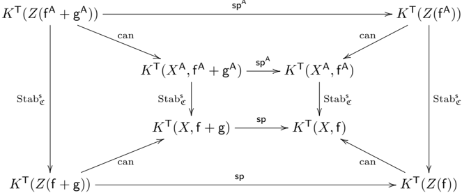
## Diagram Type: Commutative Cube Diagram in K-Theory ### Overview This image presents a three-dimensional commutative diagram, often referred to as a commutative cube, from the field of mathematics, likely specifically algebraic K-theory or a related area. The diagram illustrates relationships between eight different K-theory groups (the vertices of the cube) connected by various homomorphisms (the edges of the cube). The commutativity implies that any two paths of arrows starting from the same object and ending at the same object yield the same composition of maps. ### Components and Flow The diagram consists of eight objects (vertices) and twelve morphisms (arrows). The objects are K-theory groups, denoted by `K^T(...)`. The morphisms are labeled `sp^A`, `sp`, `Stab_C^s`, and `can`. #### Vertices (Objects) The eight vertices are arranged in two planes, a "top" plane and a "bottom" plane, each with a "front" and "back" row. * **Top-Back-Left:** `K^T(Z(f^A + g^A))` * **Top-Back-Right:** `K^T(Z(f^A))` * **Top-Front-Left:** `K^T(X^A, f^A + g^A)` * **Top-Front-Right:** `K^T(X^A, f^A)` * **Bottom-Back-Left:** `K^T(Z(f + g))` * **Bottom-Back-Right:** `K^T(Z(f))` * **Bottom-Front-Left:** `K^T(X, f + g)` * **Bottom-Front-Right:** `K^T(X, f)` #### Edges (Morphisms) The edges connect these vertices and are labeled as follows: **Horizontal Maps (Specialization):** * **Top-Back:** From `K^T(Z(f^A + g^A))` to `K^T(Z(f^A))`, labeled `sp^A`. * **Top-Front:** From `K^T(X^A, f^A + g^A)` to `K^T(X^A, f^A)`, labeled `sp^A`. * **Bottom-Back:** From `K^T(Z(f + g))` to `K^T(Z(f))`, labeled `sp`. * **Bottom-Front:** From `K^T(X, f + g)` to `K^T(X, f)`, labeled `sp`. **Vertical Maps (Stabilization):** * **Back-Left:** From `K^T(Z(f^A + g^A))` to `K^T(Z(f + g))`, labeled `Stab_C^s`. * **Back-Right:** From `K^T(Z(f^A))` to `K^T(Z(f))`, labeled `Stab_C^s`. * **Front-Left:** From `K^T(X^A, f^A + g^A)` to `K^T(X, f + g)`, labeled `Stab_C^s`. * **Front-Right:** From `K^T(X^A, f^A)` to `K^T(X, f)`, labeled `Stab_C^s`. **Diagonal/Depth Maps (Canonical):** * **Top-Left:** From `K^T(Z(f^A + g^A))` to `K^T(X^A, f^A + g^A)`, labeled `can`. * **Top-Right:** From `K^T(Z(f^A))` to `K^T(X^A, f^A)`, labeled `can`. * **Bottom-Left:** From `K^T(Z(f + g))` to `K^T(X, f + g)`, labeled `can`. * **Bottom-Right:** From `K^T(Z(f))` to `K^T(X, f)`, labeled `can`. ### Detailed Analysis of Commutativity The diagram's structure implies that all six faces of the cube are commutative diagrams. 1. **Top Face:** The composition `can ∘ sp^A` (from `K^T(Z(f^A + g^A))` to `K^T(X^A, f^A)`) is equal to `sp^A ∘ can`. 2. **Bottom Face:** The composition `can ∘ sp` (from `K^T(Z(f + g))` to `K^T(X, f)`) is equal to `sp ∘ can`. 3. **Left Face:** The composition `Stab_C^s ∘ can` (from `K^T(Z(f^A + g^A))` to `K^T(X, f + g)`) is equal to `can ∘ Stab_C^s`. 4. **Right Face:** The composition `Stab_C^s ∘ can` (from `K^T(Z(f^A))` to `K^T(X, f)`) is equal to `can ∘ Stab_C^s`. 5. **Back Face:** The composition `Stab_C^s ∘ sp^A` (from `K^T(Z(f^A + g^A))` to `K^T(Z(f))`) is equal to `sp ∘ Stab_C^s`. 6. **Front Face:** The composition `Stab_C^s ∘ sp^A` (from `K^T(X^A, f^A + g^A))` to `K^T(X, f)`) is equal to `sp ∘ Stab_C^s`. ### Interpretation This diagram likely illustrates the compatibility of several types of maps in equivariant K-theory (`K^T`). * The objects `K^T(...)` are K-theory groups associated with certain spaces or pairs, possibly involving group actions (indicated by the `T` superscript) and potentials or functions (`f`, `g`, `f^A`, `g^A`). The notation `Z(...)` and `(X, ...)` suggests different geometric constructions, perhaps related to zero loci or relative K-theory. * The maps `sp` and `sp^A` are likely **specialization maps**, relating a general situation (involving `f+g` or `f^A+g^A`) to a more special one (involving only `f` or `f^A`). * The maps `Stab_C^s` are likely **stabilization maps**, relating the theory for a space `X^A` (or `Z(...)`) to the theory for a base space `X` (or `Z(...)`), possibly involving a vector bundle or a representation, indicated by the subscript `C` and superscript `s`. * The maps `can` are **canonical maps**, representing natural transformations between different K-theory constructions (e.g., from the K-theory of a zero locus `Z` to the relative K-theory of a pair `(X, ...)`). The commutativity of the cube asserts that these three types of operations—specialization, stabilization, and the canonical comparison—are compatible with each other. For example, specializing and then stabilizing is the same as stabilizing and then specializing.

## Diagram: Transformation and Stability Relationships ### Overview The diagram illustrates a network of transformations and stability conditions between various mathematical or computational components. It uses labeled arrows to denote possible transitions ("can"), specific operations ("sp^A", "sp"), and stability constraints ("Stab^ε"). The structure suggests a hierarchical or layered system with dependencies between nodes. ### Components/Axes - **Nodes**: Represent transformed states or functions: - `K^T(Z(f^A + g^A))` - `K^T(X^A, f^A + g^A)` - `K^T(X^A, f^A)` - `K^T(X, f + g)` - `K^T(X, f)` - `K^T(Z(f))` - **Arrows**: - **Horizontal**: Labeled "can" (possibility), "sp^A" (operation A), or "sp" (generic operation). - **Vertical**: Labeled "Stab^ε" (stability condition). - **Flow Direction**: Top-to-bottom hierarchy with branching paths. ### Detailed Analysis 1. **Top Layer**: - `K^T(Z(f^A + g^A))` connects to: - `K^T(X^A, f^A + g^A)` via "can". - `K^T(Z(f^A))` via "sp^A". - `K^T(X^A, f^A + g^A)` connects to: - `K^T(X^A, f^A)` via "sp^A". - `K^T(X, f + g)` via "Stab^ε". 2. **Middle Layer**: - `K^T(X, f + g)` connects to: - `K^T(X, f)` via "sp". - `K^T(Z(f))` via "can". 3. **Stability Constraints**: - Vertical "Stab^ε" arrows link: - `K^T(X^A, f^A + g^A)` → `K^T(X, f + g)`. - `K^T(X^A, f^A)` → `K^T(X, f)`. ### Key Observations - **Branching Logic**: Nodes split into multiple paths based on operations ("sp^A"/"sp") or stability conditions. - **Stability as a Filter**: "Stab^ε" acts as a gatekeeper between layers, restricting transitions unless conditions are met. - **Operation Hierarchy**: "sp^A" appears in higher layers, while "sp" dominates lower layers, suggesting a progression from specialized to general operations. ### Interpretation This diagram likely models a system where transformations between states (`K^T`) depend on: 1. **Operational Context**: "sp^A" (A-specific operations) in upper layers vs. "sp" (general operations) in lower layers. 2. **Stability Requirements**: Vertical "Stab^ε" constraints enforce compatibility between transformed states. 3. **Possibility vs. Necessity**: "can" indicates optional paths, while "sp^A"/"sp" denote mandatory operations. The structure implies a layered optimization or validation process, where higher-level transformations (`X^A`, `f^A`) must satisfy stability conditions before propagating to simpler forms (`X`, `f`). The absence of numerical data suggests this is a conceptual framework for analyzing dependencies in a mathematical or computational system.