## Diagram: Commutative Diagram of K-Theory
### Overview
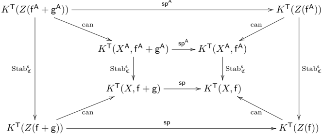
The image is a commutative diagram illustrating relationships between different K-theory groups. It shows how various maps (denoted by arrows) connect these groups, with labels indicating the specific transformations or operations being applied.
### Components/Axes
The diagram consists of the following components:
* **Nodes:** These represent K-theory groups, labeled as:
* `K^T(Z(f^A + g^A))` (top-left)
* `K^T(Z(f^A))` (top-right)
* `K^T(X^A, f^A + g^A)` (center-left)
* `K^T(X^A, f^A)` (center-right)
* `K^T(X, f + g)` (middle-left)
* `K^T(X, f)` (middle-right)
* `K^T(Z(f + g))` (bottom-left)
* `K^T(Z(f))` (bottom-right)
* **Arrows:** These represent maps between the K-theory groups, labeled as:
* `sp^A` (top horizontal arrow)
* `can` (diagonal arrows from top corners to center nodes)
* `Stab_e^s` (vertical arrows from center nodes to middle nodes, and from top-right to bottom-right, and top-left to bottom-left)
* `sp` (horizontal arrow from middle-left to middle-right, and bottom horizontal arrow)
* `can` (diagonal arrows from middle nodes to bottom corners)
### Detailed Analysis or Content Details
The diagram shows the following relationships:
1. `K^T(Z(f^A + g^A))` maps to `K^T(Z(f^A))` via `sp^A`.
2. `K^T(Z(f^A + g^A))` maps to `K^T(X^A, f^A + g^A)` via `can`.
3. `K^T(Z(f^A))` maps to `K^T(X^A, f^A)` via `can`.
4. `K^T(X^A, f^A + g^A)` maps to `K^T(X^A, f^A)` via `sp^A`.
5. `K^T(X^A, f^A + g^A)` maps to `K^T(X, f + g)` via `Stab_e^s`.
6. `K^T(X^A, f^A)` maps to `K^T(X, f)` via `Stab_e^s`.
7. `K^T(Z(f^A + g^A))` maps to `K^T(Z(f + g))` via `Stab_e^s`.
8. `K^T(Z(f^A))` maps to `K^T(Z(f))` via `Stab_e^s`.
9. `K^T(X, f + g)` maps to `K^T(X, f)` via `sp`.
10. `K^T(X, f + g)` maps to `K^T(Z(f + g))` via `can`.
11. `K^T(X, f)` maps to `K^T(Z(f))` via `can`.
12. `K^T(Z(f + g))` maps to `K^T(Z(f))` via `sp`.
### Key Observations
* The diagram is structured in a square-like fashion, with two rows and two columns of K-theory groups.
* The maps `sp^A` and `sp` appear to represent some form of specialization or projection.
* The maps `can` likely represent canonical maps or inclusions.
* The maps `Stab_e^s` likely represent stabilization maps.
### Interpretation
The diagram illustrates the relationships between different K-theory groups under various transformations. The commutativity of the diagram implies that the composition of maps along different paths between the same starting and ending points yields the same result. This suggests that the diagram represents a well-defined structure in K-theory, where the different maps are compatible with each other. The specific meaning of the maps `sp^A`, `sp`, `can`, and `Stab_e^s` would require further context within the field of K-theory. The diagram likely demonstrates how different constructions in K-theory are related and how they interact with each other.